Here is a little trick for matching two values against a two column table.
It’s much like creating a hash code for each row, then matching the hash code.
With this spreadsheet, the top section allows lookup, the lower section is the lookup table.
Here we are searching for a Value by looking up a City and Season:
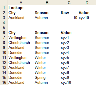
The array formula in cell C3:
=MATCH(A3 & CHAR(1) & B3, A7:A16 & CHAR(1) & B7:B16, 0)
Enter the formula by pressing Ctrl+Shift+Enter.
The formula in cell D3:
=INDEX(C7:C16, C3)
We simply concatenate A3 and B3 to match against concatenated A7:A16 and B7:B16.
The CHAR(1) is to ensure uniqueness.
For example: “userdata” & “base” would also match “user” & “database”
Fixed by: “userdata” & CHAR(1) & “base” does not match “user” & CHAR(1) & “database”
Update:
Daniel M points out a different, more efficient, match lookup using boolean comparison:
The array formula in cell C3:
=MATCH(1, (A3=A7:A16) * (B3=B7:B16), 0)
Enter the formula by pressing Ctrl+Shift+Enter.
D3 remains the same.
This works because…
A3=A7:A16 results in an array of TRUE, FALSE values
Arithmetic on a boolean results in a number. eg. TRUE * FALSE = 0.
Only TRUE * TRUE will result in the “1? MATCH is looking for.
Thanks Daniel!