It is possible to change a Chart’s Source Data by resizing individual Chart Points.

Let’s say you’ve got a Column Chart and you want to change one of the column sizes.
Click once on the column. This selects the Series. Click again on the column. This selects the single column (Series Point).
It’s not a double-click… but a click-wait-click action.

You’ll notice some blobs appear at the corners of the column.
An extra one is also positioned at the top of the column – this blob is special.
You can click-drag it to resize the column and it will change the Source Data.

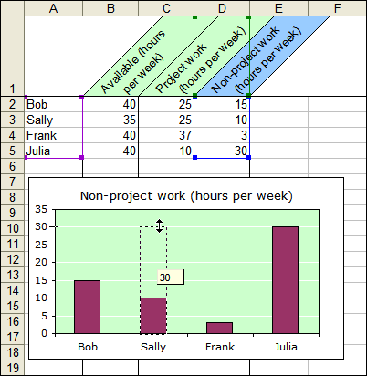
In the following example, there are some people who work a number of hours per week, of which a portion of that time is devoted to projects.
I’ve graphed the formula column non-project work. The formula in D2 is =B2-C2

I can hear you saying:
Hey! When you resize that column, it’s going to overwrite your formulas!

Excel is pretty smart and knows it’s a formula, so it throws up Goal Seek.

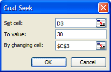
In this case I’ve told Goal Seek to keep changing the “Project hours” until “Non-Project hours” becomes 30.
Project hours gets set to 5 and we’re happy!