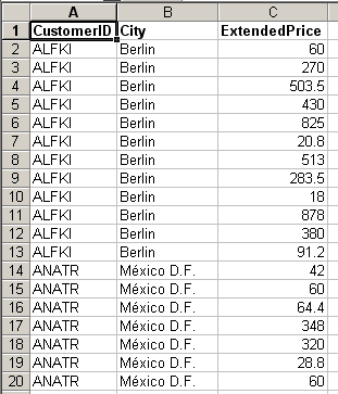
Pivot tables can be used to summarize data in interesting ways. In this example, I start with selected data from the Invoices table of Northwind.mdb. The table contains 2,156 rows, each representing one invoice. The selected data is the Customer ID, City, and Extended Price. I want to see the sales by City.
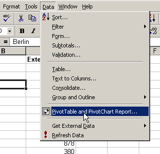
Select a cell in the table and choose PivotTable and PivotChart Report… from the Data menu
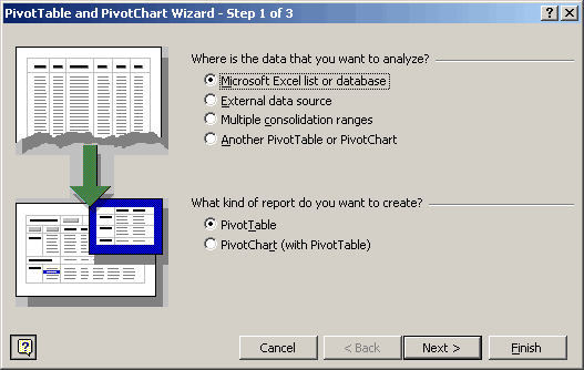
Step1 allows you to select where to get the data and what kind of report to produce. We’ll be using an Excel table and producing a Pivot Table.
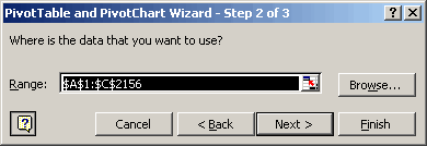
With a cell from the table selected, Excel will guess what the whole table is. You need to have a header row for your data, the value of which you will see in later steps. If Excel doesn’t guess correctly, you can change the range in this step. You can also select the entire range before starting the wizard to help Excel guess correctly.
The final step of the wizard allows you to define where the table will be created, either on an existing sheet or a new sheet. For this example, I’ll choose New Sheet.
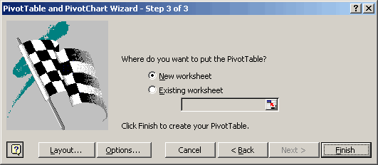
This step also provides a Layout button and an Options button. You can define the rows and columns of your table using the Layout button or just click finish and define them on the worksheet. I’ll choose to define them directly on the new table as opposed to using the Layout button. By clicking finish, Excel creates the table and displays the skeleton.
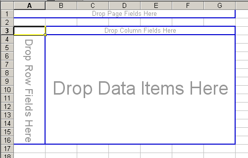
The Pivot Table toolbar shows all the fields from the Excel list, from which you can define the layout of the table. The three fields Customer ID, City, and Extended Price are shown as buttons on the toolbar.

To define the layout, drag the City button to the area that says “Drop Row Fields Here” and drag the Extended Price button to the “Drop Data Items Here” area.
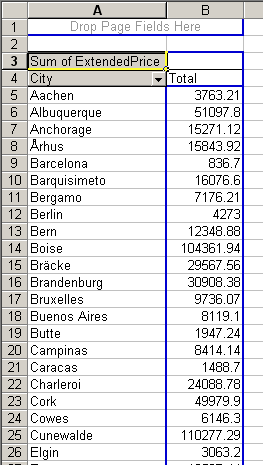
Excel guesses what you want to do with the Data Items. In this case, since Extended Price is a number, it guesses that you want to Sum them and creates the Sum of Extended Price data item. If you don’t like Excel’s guess, you can change it by right clicking on Sum of Extended Price and choosing Field Settings.
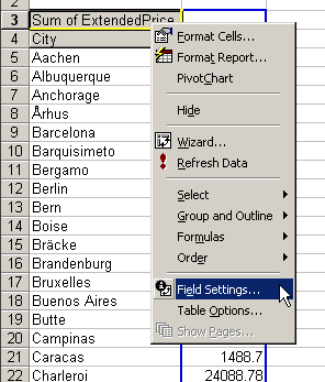
Change the Summarize By listbox to Count
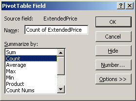
to see the number of invoices by city instead of the total sales.
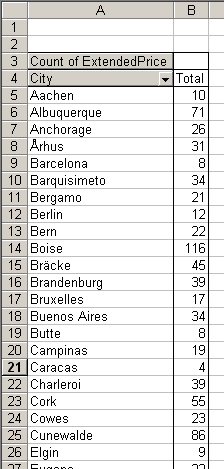
That’s the basics of creating a simple pivot table. There are a lot more options and much more that you can do with pivot tables, which I will cover in future posts.
Someday…someday! I will get these things figured out.
Thanks for the help.
Hi Dick,
At work I find Pivot tables great, but the greatest feature ever I found in one of JWalk’s books: to summarize a list using Data – Table (I haven’t got the book here, but I believe it’s around page 268 in Excel Formulas).
Pivot tables are quick, and they allow you to ‘slice and dice’ the data in any way you want, but you have to keep making new pivot tables each time your list is updated. Most of the time that doesn’t really matter, but what if you work with a permanent list which is updated several times a day?
A ‘data table’ refreshes the data in your list automatically, because it considers the source data list as an array. As JWalk says it: pure magic.
However, please continue blogging about Pivot Tables; I’m sure you’ll get an awful lot of comments!
Frank.
P.S. My statistics teacher found a I found a bug with sorting in Pivot Tables; I’ll comment on it later.
Willson –
You just have to play with pivot tables a bit. Suddenly you’ll get it, and you’ll use them forever.
Frank –
Define a dynamic named range that includes the pivot table source data, and changes size as the data range changes. Go to the Inser menu, Names submenu, Define item (or the shortcut CTRL-F3), enter a name like PivotData1, and in Refers To, enter a formula like:
=OFFSET(A1,0,0,COUNTA(Sheet1!A:A),COUNTA(Sheet1!1:1))
When defining the source data for your pivot table, enter the defined name PivotData1. Whenever you update the pivot table, it will use the updated definition of PivotData1, and therefore use all of the data.
Don’t wait too long with your bug report.
Dick –
A nice introduction. I have several clients whose projects were best carried out by automating pivot tables. Often they ask for background information, so I’ll add this to the list of web pages I reference.
– Jon
Jon, the bug my teacher was talking about must be in a version previous to Excel 2000, because I repeated his experience and found no sorting errors. Here is what he found anyway:
When column or row labels consist of only one character, the pivot table sorts (*) any longer labels after the one-character ones. From his source table with regions a, b, b23 and c, the sorted labels in the pivot table came out a, b, c, b23.
(*) In Dick’s example, the row labels correspond to the cities in the source table. If we wanted the pivot table to sort them in a particular order, for example descending, we would right click the City Row Field, select Field Settings, select Advanced, and choose Descending in the AutoSort options.
Great post… I’ve recently started to become “almost” proficient with Pivot tables. These are incredibly powerful once you start to understand how to use them. Please keep up the posts. I’m thrilled to have come across this site. I’m sure I’ll be visting frequently.
Kent
Frank –
I’ve never come across that one, and I used Pivot Tables in 97 a great deal. My problem was with long labels, though, which made the table hard to read. I’m glad you can no longer reproduce it.
Kent –
Just keep on using the suckers, and before you know it, you’ll be an expert.
– Jon
I loath pivot tables with a passion, largely because of the need to refresh them. I’m very absent-minded so the risk of reading off the wrong result just because I forgot the intermediate step is too great.
Also, they’re inherently very unsuitable as an intermediate step in a calculation; GETPIVOTDATA is the worst formula in Excel so god help those using Excel 2000 and below. That cute little knack they have of overwriting other data on your worksheet when their size expands gets me too.
I suppose fundamentaly I can never see any reason WHY I should use them when ordinary worksheet formulas can do the same functionality, maintain an audit trail much better and calculate automatically – I can never remember to refresh the damn things when i change the input data.
Jon-
A pivot table referring to a dynamic name – thanks for this cool tip.
There still seems to be something that a pivot table can’t do, unless I’m completely wrong.
Suppose that in Dick’s source table there is a fourth column: ExtendedPriceVatInc, for example.
How do I obtain a table with as many rows as there are cities (like Dick shows in the post above) with not one, but three summary figures per city?
1) the number of invoices
2) the sum of ExtendedPrice
3) the sum of ExtendedPriceVatInc.
Charly-
A data table, once it’s set up, always shows the exact summary of your source table. Only your throat will ever need refreshments. I’ll keep you posted.
Frank-
Frank –
Add all three fields to the data area, then grab the button for the data area, and drag it from the row area to the column area.
Charlie –
You can put a line of code in the Workbook_Open and Worksheet_Change to refresh the pivot table automatically; also use a defined dynamic name for the source data, as I suggested to Frank a couple posts ago. I suppose if the table might grow large enough to engulf other data, you could build it on its own worksheet (I like them with other data, though, too). And I didn’t even know about the Get Pivot Data functions until recently. I use other worksheet formulas that don’t know it’s a pivot table, or I use VBA, and everything works so nicely.
– Jon
Jon-
I can do with a refreshment when I see how easy it is!
Charly-
To summarize the situation: you have the choice between an automatically refreshed pivot table, based on a dynamic named range, or a data table that works with an array formula.
I think the simplest is still a spreadsheet (non-VBA) solution; naming the source data dynamically is just as great for pivot tables as it is for a data table.
-Frank
Jon – using formulas other than GETPIVOTDATA to reference cells in a pivot table is, for me, far too risky as the reference does not move when the table resizes, potentially rendering all of your formulas incorrect. That’s a good point you make about the worksheet_change event though, I will use that in future.
Frank – I’m a fan of data tables too, though they do have the drawback of serious performance overhead on a complex model; of course, I could set the calculation mode to exclude tables but then I’d have to remember to press F9, which kind of leaves me back where I started…
Charlie
Charlie –
The moving references merely make the analysis of the pivot table more interesting. What helps is to move the pivot table down and right, put the formulas above and left of the table, and nothing at all below or right of the table. Alternatively, put the PT on its own sheet, and formulas on the next sheet. You can use Count and Counta to help figure out the regions of the PT.
Of course, using VBA enables you to directly access the field ranges, which is as robust and more flexible than the GETPIVOTDATA seems to be.
– Jon
What would be the best book or reference material for someone new to Pivot Tables to really get up to speed fast using these? My new job will require me to know what I’m doing. I’ve been playing with examples and using Excel Help and reading up on websites but want to purchase a book to refer to so your suggestions would be most welcome. Thanks!
I’ve never read a book that was that narrowly scoped, but you should check here
Contextures Book List
There might be something under Special Interests.
There’s a book on pivot tables, by Cornell, published by APress. I noted it in Borders a couple weeks ago but didn’t rate it the way I usually do, and I can’t remember what it was like.
Walkenbach’s Excel Bible and Excel Formulas both have decent PT chapters (probably the same chapter). I’d recommend the Bible because of the breadth of its other content, unless you really need formulas.
Excel Data Analysis by Simon has a PT chapter with lots of screen shots, to give a more visual description. It may not be as rigorous a coverage as Walkenbach’s.
Finally, get yourself some good sample data, and play around. Get right into the form and drag the buttons around and see what you can do. See what effect moving buttons and fields has on the structure of the table and the arrangement of the data. There’s no replacement for a subconscious sense for how these things work.
– Jon
http://www.1keydata.com/datawarehousing/dimensional.html/
http://www.rkimball.com/
Pivot Tables For Dummies.
Excel is neither a data warehouse tool nor is it a statistical package, yet interestingly it has functionalities of both.
Practical people ask ìhowî, only dummies ask ìwhyî. But I wanted to know more about Pivot Tables without having to go through a long process of trial and error. So I left any mathematic intuition aspects aside, and went for some background. I ended up in the context of dimensional data modelling (DDM) and decision support systems (DSS). This is a way of thinking that has been around for decades, and that is used in data warehousing. The following points will be revision for most of you, but dummies will love it:
Point 1.
A Pivot table must be based on a flat database, i.e. a table with headers in the top row and “records” below. This is not always obvious ñ it can be hard work to get your data in that form (data cleaning is not a joke) but once it is, youíre half way there.
Point 2.
In your ìflat databaseî or source table, there really are only two types of data: factual and dimensional data.
Point 3.
The data you want to summarize are usually the factual data: they are numeric and continuously valued. Summaries of non-numeric or discontinuously valued data (Count, Min, Max) are less powerful.
Point 4.
The dimensional data are the actual drivers of the data analysis. Each dimension (e.g. time, region, product) can have several attributes (e.g. month, quarter, year for the time dimension). These data are discretely valued, usually alphabetic.
So there is at least one move in the making of a pivot table that need not be an act of subconscious wizardry: to drag the numeric fields you want to summarize from the Pivot Table toolbar to the area that says ìDrop Data Items Hereî. But apart from that, drag as many data fields into the row and/or column areas as you like, pronounce a magic formula, juggle everything around, including the numeric fields you just dragged into the data area, and ñ hey presto. If you donít like the result, start again.
A ìfact tableî in a data warehouse typically has hundreds of columns and millions of records. DDM and DSS software, developed for managers to analyse their business data, is still quite professional and inaccessible. Just like MS Access in the opinion of countless Database professionals, Excel Pivot Tables are only a toy, but if you donít play, you donít learn!
P.S. Another book that talks about Pivot Tables is Excel Data Analysis For Dummies. Curiously, it also discusses the Excel statistical functions in great detail.
Is it possible at all to link two pivot tables. My data set has the following fields: Sales person, Product, Customer, Sales volume and revenue. I have this data for 3 years in seaprate data sets and would like to generate a pivot table report where I can get to sales by person, by product and by customer for the three years (laid out one below the other, ie three lines for each year of data). It it possible at all to link pivot tables?
I have tried merging the three years data by inlcuding a field for the year, but am unable to make it work. Any suggestions would be most appreciated!!
Thanks
AD
Aditya, you are right about wanting to merge your data into one table and about adding an extra field for the year. It is much easier to make 3 reports out of one table than to make one report based on three separate ones. Once you have managed to make this table with the 6 column headers and any number of records up to 65535, create a simple Pivot Table with Sales Person in the row area, Year in the column area and Sales Volume in the Data Items. Same procedure for Customer and Product.
As mentioned the GetPivotData function, which promises so much, can appear to be worse than useless, especially if the items that appear in the row/column fields are not very long or are numbers.
The help for the function in XL97 suggests you use this kind of syntax:
GETPIVOTDATA(A4,”March Buchanan Produce”)
..but I find this often does not work and returns errors or the wrong values.
However, if you surround the item value you are looking for in single quotes and square brackets and include the actual row/column field name, the problems with GetPivotData seem to evaporate.
=GETPIVOTDATA(A4,”month [‘March’] salesperson[‘Buchanan’] product [‘Produce’]”)
This format seems to work no matter what I have thrown at it (famous last words…) so it may be worth trying if you are having problems. As usual, you can build the search string by concatenation so you could look up pivot data based on values that have been, for instance, type into a cell.
I’m using a named range in a workbook and referencing this from the Pivot Table that is in another workbook.
What I find is that ‘dynamic data’ (i.e. VLOOKUP) is not passed through to the Pivot Table.
Any suggestions as to how it can be incorporated?
the article on pivot table was really good as it gave me an introduction to pivot table’s. i Will try using it and then see wether its reall y that complicated as it seems.Thanks for the information
Hi
I am trying to run a vlookup on the results of a pivot table but it is not working. I have also tried copying the data out the pivot using Getpivotdata but the vlookup won’t work on this either.
Any ideas what the cause might be?
(I have made pivot tables and vlookups before and I know that these would work on a static data but somehow I can’t combine them)
Thanks
Tim
You saved my life, that was extremely helpful,thank you!!!! all the best and waiting for your new publications
How can I count the unique values with pivot table?
Maggy
Is there a way to use Data Field items in a pivot table without the gaudy GETPIVOTDATA function?
EG. Use =B7-B8 instead of
=GETPIVOTDATA(“Average of AdjPrice”,$A$3,”Location”,”AVOC”)-GETPIVOTDATA(“Average of RMV”,$A$3,”Location”,”AVOC”)
OR
=1/B6 instead of
=1/GETPIVOTDATA(“Average of Ratio”,$A$3,”Location”,”AVOC”)
Like it was in XL 2000. GETPIVOTDATA function sucks big time!
doco
I must be doing something wrong. I have a dynamic range ‘sales_analysis’ and placed that name in the ‘Range’ TextBox on Page 2 of 3 on the wizard, but get this error
doco
doco,
> Is there a way to use Data Field items in a pivot table without the gaudy GETPIVOTDATA function?
>
> =1/B6 instead of
> =1/GETPIVOTDATA(ÄùAverage of RatioÄù,$A$3,ÄùLocationÄù,ÄùAVOCÄù)
There may be a better way, but when EXCEL inserts the GETPIVOTDATA() function, you could:
Hold down the shift key
Move the cursor key left or right (this changes GETPIVOTDATA() back to a range like “B6:C6?)
Hit the backspace keys to delete off the “:C6? suffix that was added
Hit enter (or continue with creating your formula)
But keep in mind that your references may become invalid if the Pivot Table gets refreshed and the dimensions of the table change.
doco –
“Is there a way to use Data Field items in a pivot table without the gaudy GETPIVOTDATA function?”
You just have to type the addresses by hand.
There’s a toggle for GetPivotData selection which can turn it off.
Go to Tools|Customise then click data on the commands tab and scroll to the bottom of the list -then drag the “Generate GetPivotData” onto a toolbar. Selecting this determines whether clicking a cell in a pivottable returns a simple reference or a GetPivotData formula.
hughbert-
>The help for the function in XL97 suggests you use this kind of syntax:
>GETPIVOTDATA(A4,ÄùMarch Buchanan ProduceÄù)
>..but I find this often does not work and returns errors or the wrong values.
I CANNOT AGREE MORE!
>However, if you surround the item value you are looking for in single quotes and square brackets >and include the actual row/column field name, the problems with GetPivotData seem to evaporate.
>=GETPIVOTDATA(A4,Äùmonth [ÄôMarchÄô] salesperson[ÄôBuchananÄô] product [ÄôProduceÄô]Äù)
>This format seems to work no matter what I have thrown at it (famous last wordsĶ)
I have thrown some fields with a single quote(s) in their name:
This strategy fails as well!
eg. Try with: Buch’anan
But remove the single quotes in your square brackets and that issue get’s solved as well!
=GETPIVOTDATA(A4,Äùmonth [March] salesperson[Buchanan] product [Produce]Äù)
I understand that a Pivot Table summarizes the data, but what if I have a field for example like “Description” which holds a bunch of characters. When I use Pivot Table it does not list all the characters from the source data. It cuts off to certain point since in theory it is summarizing it. Is there a way to turn the summarizing off to allow a particular field to display all the values of the field from the source data?
In my part of the world there is confusion about the way you pronounce the word ‘pivot’ in pivot tables. Some pronounce the [i] like in ‘fish’, others pronounce it like in ‘dive’. The word is too recent to appear in a dictionary. Could anybody Anglo-saxon remove our doubts?
Frank –
Here in America (oh, I don’t mean to sound pretentious), both vowels have about the same sound, except for the accent on the first. So, “i” as in “fish”.
– Jon
>> The word [pivot] is too recent to appear in a dictionary.
Frank,
You might consider putting that dictionary you are using on eBay. The verb “to pivot” is recorded as early as 1841, from the noun “pivot” meaning “central point” that goes back to at least 1813. Online, the word “pivot” can be found in Webster’s 1828 dictionary.
It’s also in the more recent Merriam-Webster’s at this link: http://www.m-w.com/cgi-bin/dictionary?book=Dictionary&va=pivot, where you can hear the word (or any other) aloud.
Microsoft introduced the term “Pivot Table” with version 5 of Excel in October 1993. The functionallity was similar to earlier “Cross Tab” functions in Lotus and other products, but now you could “pivot” data in the report, i.e. easily move a column sub-heading to a higher level. So if you had Sales by Month by Sales Person, you could click-and-drag to pivot on Month and instantly see Sales by Sales Person by Month.
David
Doco,
I agree that the “getpivottable” function sucks.
for example, in XL2000 I used to create a difference column on
the right of the pivottable like “B3-A3?.
Excel 2003 “translates” this into
=+GETPIVOTDATA(“Amount”;$A$3;”SALES”;”SALESNOVEMBER”;”Cat1?;13)-GETPIVOTDATA(“Amount”;$A$3;”system”;”SALESOCTOBER”;”Cat1?;13)
And it doesn’t work. All it shows are zero’s, not the difference.
So I generally copy the whole pivottable and paste it “as values”, and then proceed as i
always did before, by clicking b3 – a3, and pulling the formula down
But thanks for the tip on how to toggle off this bogus formula.
Andreas
I am having a problem with getting my pivot table to take in a dynamically named range (created using an offset).
I put the name of the range (primary_1D) into the Range field (on step 2 of 3) in the make a pivot table wizard, but it comes up with the error ” The pivot table field name is not valid. To create a pivot table report, you must use data that is organized as a list wiht labelled columns. If you are changing the name of a pivot table field, you must type in a new name for that field.”, even thought the data is in a list (5 headings across, 28 rows down). I can’t use a static address, because the length of the range is always changing.
Could the blank row at the end of the list (in the dynamically named range) be the problem? If so, how can I get rid of it? It doesn’t matter what the naem of the dynamically named range is (I tried it using Database as well).
Alternatively, how can I get my Pivot table not to display “(blank)” in blank cells.
Any help is greatly appreciated.
Liz, I think the problem may be with one of your column headers (i.e., field names). My guess is that one of them is blank. And that’s probably the column that you use to count the rows — which explains why your dynamically generated name has an extra row.
Has anyone experimented with the “Calculated Field” functionality of the pivot table? It seems quite powerful, but (as usual) is missing that one little piece of functionality that I need. I want to use the total of a column in a calculated field, but the “SUM” function doesn’t seem to make that happen. Any thoughts? For example, you could re-generate the “% of column” by having the formula be =column / SUM(column).
If anyone has any suggestions, I’d really appreciate it Thanks!
Hello all – forgive me if this has been covered but I’m new to the site and still feeling my way around…..I use Office Pro 2003 and recently wrote the following for my wife to automate what was before a fairly tedious process of generating 2 pivot tables – which works fine, except that her computer runs Office Pro 2000. My “problem” is that Excel 2000 seems not to support the line of code :ActiveWorkbook.ShowPivotTableFieldList = False, as a result of which whilst the program runs ok and achieves the correct result, she has to keep closing (twice per execution) the dialog boxes for pivot table field names.
Does anyone know a workaround for this please! (other than upgrading her computer to office 2003….?!)
thanks
‘ Create a skeleton of a PivotTable
Set pvtTable = wksData.PivotTableWizard(SourceType:=xlDatabase, _
SourceData:=rngData, TableDestination:=wksDest.Range(“B5?))
‘Close the PivotTable Field List that appears automatically
ActiveWorkbook.ShowPivotTableFieldList = False
‘Add fields to the PivotTable
With pvtTable
.PivotFields(“SITE”).Orientation = xlRowField
With .PivotFields(“LOG”)
.Orientation = xlDataField
.Function = xlSum
End With
End With
‘Autofit columns so all headings are visible
wksDest.UsedRange.Columns.AutoFit
‘ Next Pivot table
‘ Set up object variables
Set wksData = ThisWorkbook.Worksheets(“Filtered Data”)
Set rngData = wksData.UsedRange
Set wksDest = ThisWorkbook.Worksheets(“Pivot Tables”)
‘ Create a skeleton of a PivotTable
Set pvtTable = wksData.PivotTableWizard(SourceType:=xlDatabase, _
SourceData:=rngData, TableDestination:=wksDest.Range(“E5?))
‘Close the PivotTable Field List that appears automatically
ActiveWorkbook.ShowPivotTableFieldList = False
‘Add fields to the PivotTable
With pvtTable
.PivotFields(“SITE”).Orientation = xlRowField
With .PivotFields(“DIGEST”)
.Orientation = xlDataField
.Function = xlCount
End With
End With
‘Autofit columns so all headings are visible
wksDest.UsedRange.Columns.AutoFit
[…] any help: Daily Dose of Excel ª Blog Archive ª Creating a Simple Pivot Table […]
Can I merge two pivot tables into 1? How can this be done?
Thanks.
hi
I would like to know how one can consolidate the data from two pivot tables
I am using the GETPIVOTDATA function to pull info from a pivot table I update on a weekly basis. The problem I am having is that I am pulling info based on a dept and job number however that job number might not be listed in the updated information so I am getting #REF! error. To correct it I have to go through the information and remove that GETPIVOTDATA function or add it is there a way to setup so I don’t receive the error when the job number is not listed?
Thanks.
If a pivot table in Excel gives a count like 10 and if you run the sum it gives zero’s what is the problem
Very helpful indeed! Thanks!
I just starting learning pivot tables and thought they were great until I encountered this baffling problem. I am sure the fix is obvious, but I can not figure it out.
After dragging and dropping a field to the table, it no longer keeps a count or grand total. This basic function was working beautifully yesterday, and today it is not working. I double-clicked on the heading and it is set to automatic. I also checked the options and both the rows and columns are set to show totals.
Help!
I have over 40 pivot tables that are based on data connected to a view in SQL server database. We then changed 90% of the field names in the SQL database – e.g. FuelDomain changed to EvalFuelDomain and MeasureDesc changed to PrgTrkMeasureDesc. When I updated the view in excel, almost all the column headings(field names) that the pivot tables used got changed. Now if I refresh the pivot tables all my tables blank out – understandably so as the table is looking for the old field names.
Short of recreating each pivot table, is there a way to get the tables to use the new field names?
Help
I use pivot tables all the time but have an issue I think may be related to trying to use PT created in Excel 2003 and trying to work with them in Excel 2007- namely the data source fields keep resetting themselves.
Eg I have the table set to source all rows in Columns A-U, but when I paste in new data onto the source page, when refreshing the PT – it defaults back to a range of Rows – eg A2-U16348
I have changed the tables via the “Change Data Source” option back to read all rows in A-U but the next time I open and paste in more data – it changes back again
Any ideas
Is there anyone out there who can point me in the right direction? I have spent countless hours on this. I am reasonably adept at using pivot tables but am unable to make “if statement” syntax in a calculated field work. I link directly to an sql accounts database via MSQuery and return a very simple result to a pivot table. I wish to create a calculated VAT field to emulate the following excel if statement:- If(stock_vat_type=”G”,val*7/47,0). If I key this into my calculated field, the syntax is accepted but will not give me the result I am looking for. Help !!!!!!!!!!
Hi Jon (assuming you’re still subscribed to this thread).
You say above “VBA enables you to directly access the field ranges, which is as robust and more flexible than the GETPIVOTDATA seems to be.” Do you ever use VBA (or a non-VBA trick) to reference columns in a pivottable so that they can be charted without any errors if the pivot structure is altered a little? I.e. perhaps a non essential field is taken out, and so everything to the right of that point moves one column to the left – do you have any tricks to get your dynamic chart series formulas to rescope accordingly? I could use some VLOOKUPS and OFFSETS and the like, but I want to be able to cover the situation where a pivottable might move around by quite a few rows or columns.
What would be real cool would be to select the entire table with some VBA based on a reference from one GETPIVOTDATA field (which would update dynamically if the pivottable was shifted) then define names for the ranges using the “Create from Selection” range feature (Excel 2007)…assuming it will update or overwrite existing names created from the same pivot table. I’m just about to explore that method, but thought I’d see if I’m merely reinventing the wheel.
Any thoughts greatly appreciated.
Jeff
Just realised the answer lies in using the Getpivotdata function to pull the data outside of the pivottable into a parking space, and then use dynamic named range to reference that parking space and change the size of the array accordingly to match the actual pivot table row height. Obviously my brain needed to talk out loud to see this obvious solution….
Jeff –
The Send/Submit button is a great educator.
The thing with VBA is you can identify the whole range of the pivot table, the data range, each pivot item of each pivot field and their associated ranges, and the relevant ranges for charting using Intersect and Union. GETPIVOTDATA requires either some knowledge of the contents and structure of the pivot table or some monstrous formulas to extract this kind of data, plus a parking area that requires the flexibility to grow and shrink as needed (mostly grow). And you can’t make a dynamic chart that adds or removes series without using VBA. I guess you could have a number of dummy series which don’t appear unless there is data, but this leaves residue in the legend and messes up spacing in a clustered column chart.
Cool…it’s VBA for me then. Haven’t got to the part of Power Programming with VBA concering pivottables yet…keep alternating between Few, Walkenbach, and my bank statements, so reading is slow progress. Thanks for the overview, you’ve got me hooked on my next challenge.
On residue in the legend, how about the tried and tested “this series has been intentionally left blank”
Hey all,
I was having the problem with the (blank) ruining my pivot tables and created a macro to take care of the issue. In a nutshell, my code will run through your pivot table and change the color of the cell containing the (blank) to white, making it invisible. Please make sure you run the script after every time you update your pivot table to ensure that cells that should be white are and cells that shouldn’t aren’t.
Enjoy
Sub Remove_Blank_From_PivotTable()
‘ The purpose of this macro is to remove the word (blank) from apprearing
‘ on any pivot table report. This code is completely generic and requires only
‘ the absolute minimum amount of intervention from the user
‘ Instructions: Copy and paste this code into the VBA editor from excel into a module attached
‘ to the spreadsheet that contains the pivot table you’d like to clean up
‘ On line 33 of the code there is a variable that is used to store the name of the spreadsheet
‘ that contains the pivot table. Simply change the name and run the macro
‘ Copyright: Benjamin Crudo, August 12, 2009
‘ Please send all feedback to benjamin.crudo@gmail.com
‘ This software is free to use and redistribute by anyone who wishes to do so
‘ If you require more help with excel or other programming needs
‘ at your place of business please contact me via email for my rates
‘ Copyright: Benjamin Crudo, August 12, 2009
Dim counter As Integer ‘ setting up a counter to loop through the worksheet
Dim lastRow As Integer, lastColumn As Integer ‘ creating variables to store the last
‘ rows and column that contain data on the worksheet to limit the loop
Dim WorksheetWithPivot As String ‘ declaring a string to store
‘ the name of the sheet containing the pivot table
Dim wb As Workbook
Dim ws As Worksheet ‘ Declaring a Worksheet variable to use to
‘ access the worksheet with the pivot
‘____________________________________________________________________________________________________________________
WorksheetWithPivot = “Master Pivot” ‘ enter the name of the worksheet that contains the pivot table here
‘ replace the words “Master Pivot” with the name fo your sheet with your pivot
‘____________________________________________________________________________________________________________________
Set wb = ThisWorkbook ‘ setting the workbook object to this workbook
‘ note, if you wanted to run this script on another excel file
‘ you would change the workbook and worksheets paramters, or
‘ you could just copy and paste this code into another workbook VBA module
Set ws = wb.Worksheets(WorksheetWithPivot) ‘ setting the Worksheet object
i = 1
j = 1
lastRow = ws.UsedRange.Rows.Count ‘ locating the last row used on the sheet
lastColumn = ws.UsedRange.Columns.Count ‘ locating the last column used on the sheet
Do While i <= lastRow ‘ loop through each row that contains data
Do While j <= lastColumn ‘ loop through all of the columns in each row
If ws.Cells(i, j) = “(blank)” Then ‘ if there is a blank in the current cell make it’s text white
ws.Cells(i, j).Font.ColorIndex = 2 ‘ make the text white if the cell contains a (blank)
Else
ws.Cells(i, j).Font.ColorIndex = 1 ‘ Ensure that the text is Black if there is no (blank) in the cell
End If ‘ end the if statement
j = j + 1 ‘ increment the column
Loop ‘ loop through the columns
i = i + 1 ‘ increment the row
j = 1 ‘ reset the column counter back to 1 (the beginning)
Loop ‘ loop through the rows
End Sub
Hmm..
Obviously my brain needed to talk out loud to see this obvious solutions..
I posted this question on the Bacon Bits blog, but thought I’d ask it here. Recently I’ve created a couple of pivot tables and noticed that their file sizes are much LESS than a spreadsheet containing just the raw data. For instance, if I create 3 complete rows of =randbetween(0,10000) in excel 2007 and then convert these ranges to values, then here’s the resulting file size from those 3.14 million cells:
raw data only 26.4 MB
Pivot table only 12.6 MB
Pivot table and data 39.1 MB
The pivot table is half the size, but contains 100% of the data that can be restored with a mere double-click. This really surprises me. Anyone know why this might be?
Seems to me that if you’re going to distribute a big file, and for some reason you can’t zip it up, then stick it in a pivot table rather than email the raw data.
Jeff: My guess is that the memory requirement for storing a PivotCache is less than for storing a range. Again guessing, but I’ll bet they store far less data in a PivotCache. Maybe they have to reserve memory for things like cell comments and conditional formatting, whether or not they exist, when storing ranges that they don’t have to store for a PivotCache. There’s probably a ton of properties that just aren’t relevant to the data, but are relevant to a worksheet cell. Take the Locked property for example. That takes 2 bytes of data per cell and they wouldn’t have to store that property for data in a PivotCache.
Thanks Dick. There’s still some stuff puzzling about all this to me…check this out:
On my home pc, using excel 2007 if I create 3 complete rows of =rand() then convert them to values, then:
1: when I save the workbook, I get a file size of 50 MB.
2. If I then create a pivot table on a second sheet from this data, but don’t explode it (i.e. don’t put anything in the data or column/row areas) I get 83.6 MB for pivot and data. So it seems the pivot alone adds 34 MB.
3. If I then explode the pivot table (i.e. put all three columns in the row area) so that the pivot resembles the original data source, I get 163 MB for pivot and data, which is quite some increase. I’d expect to actually see 50 MB (raw data) plus 34 MB (Pivot Cache) plus perhaps another 50 MB MAX for the extra resource required to store the cell formatting info for the range used by the exploded pivot. So the most I’d expect this to take up would be 134 MB, but it runs to 163 MB.
4. If I delete the raw data on Sheet 1, the file size drops 50 MB to 113 MB for the exploded pivot only, as you’d expect.
5. If I drag the three columns out of the pivot, then I get 52 MB for the unexploded pivot – which is almost the same file size as for the data alone. (Note I deleted all cells below and to the right of the pivot in order to try to make sure excel’s used range was limited to the pivot only. Not sure that this worked, given this high file size) So my pivot only seems to have grown from a 34 MB footprint when created to 52 MB just because I exploded it then contracted it.
6. If I reopen the file from (2), delete the data, and save the unexploded pivot, I get a file size of 34 MB…which was what I was expecting in step 5.
It seems very odd that if you expand a pivot table out, then contract it, the file size doesn’t decrease accordingly.
Maybe this means that if you’re playing around with a pivot that at some time you’ve exploded, then you might want to recreate your final product from scratch to cut down on some file size.
Anyone have any thoughts on this behavior?
Thanks for this basic information to Pivot Tables. It has made me to realise that Pivot Tables could be basic and are not so complex. It has also given me the confidence that I can succumb my ‘phobia’ for Pivot Tables and become a Master of the Pivot Table. This, I am going to do! Thank you, for breaking it down so simply.
I am using the pivot table on a regurlar basis and has solved many issues.What I am struggling with the charting where for every change in the cursor movement the graph changes also.If you can help me with the step by step creation of those graph vy way of VBA CODING that will be excellent.
Kindest regards
Jacob Bokaba
Excellent explanation!

Always wanted to understand Pivot tables and here I got a very straight forward and comprehensive explanations.
Thank you very much
Hi Dick,
Excellent explanation!
I loved the example you used, it is perfect for Pivot Table newbies to understand.
I would like to share some points about how I see Pivot Table creation process…
It may help to those in trouble with “dragging what to where”.
Let me define the Pivot Table drag-and-drop areas…
1. Left drag-and-drop area: row
2. Top drag-and-drop area: column and page
3. Center drag-and-drop area: data
On the left/top areas, you have category fields: City, Customer, etc.
On the center area, you have number fields: Sales, Price, etc.
I hope it helps
Nice explanation, well done.
Pivot Table is very easy and much helpful for tables like this, well done.
I am trying to figure out how many widgets I need to order for every item listed. I have a sheet of items (rows) where for each row there may be an amount needed or not. For each row that has an amount needed, I need to create another worksheet with ONLY the rows where there is an actual requirement with the quantity needed, item name and state. Here is sample data of the listing in Worksheet A:
Name State Qty
Apples WA 5
Oranges FL
Car MI 8
Furniture VA 3
Corn IN
Notice that the Qty is empty in many of the rows. Desired output on Worksheet B:
Name State Qty
Apples WA 5
Car MI 8
Furniture VA 3
So the output does not include the empty qty records. I’ve tried various row formulas and others and am just having a hard time. I’d prefer to do this with a formula rather than macro or such and not using a filter. Any assistance would be appreciated.