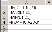
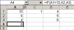
When writing complex formulas, it’s usually beneficial to build the formula by putting smaller pieces of it in several cells, then combine those cells into one long ugly formula. I’ve been thinking that I need to write a macro that does the combining for me, but like so many things, it gets on the back burner and never gets off.
Fellow MVP, Bernie Deitrick, shared a macro that he wrote and I finally decided to write mine. So this is at least partially stolen from Bernie (Thanks).
Sub BuildFormula()
Dim rPrec As Range, rAllPrecs As Range
Dim sForm As String
Dim rCell As Range
If TypeName(Selection) = “Range” Then
For Each rCell In Selection.Cells
On Error Resume Next
Set rAllPrecs = rCell.Precedents
On Error GoTo 0
If Not rAllPrecs Is Nothing Then
sForm = rCell.Formula
For Each rPrec In rAllPrecs
If rPrec.HasFormula Then
sForm = Replace(sForm, rPrec.Address(0, 0), _
“(” & Replace(rPrec.Formula, “=”, “”, 1, 1) & “)”)
End If
Next rPrec
rCell.Formula = sForm
End If
Next rCell
End If
End Sub
Here’s a simplistic example of how it works. Note that I’ve overdone it with parentheses, but better safe than sorry.


Update: Jonathon notes a bug in my macro. If both A1 and A10 are in the precedents, the A10 would be replaced by A1’s formula except for the zero. Now I remember why I never wrote this macro. Anyway, here’s another stab at it. I think converting the formula to R1C1 relative references should eliminate that problem. Please let me know if I’ve missed anything else or just made it a whole lot worse.
Sub BuildFormula()
Dim rprec As Range, rAllPrecs As Range
Dim sForm As String
Dim sNewRef As String ‘new variable to convert address to R1C1
Dim rCell As Range
If TypeName(Selection) = “Range” Then
For Each rCell In Selection.Cells
On Error Resume Next
Set rAllPrecs = rCell.Precedents
On Error GoTo 0
If Not rAllPrecs Is Nothing Then
‘Convert the formula to relative R1C1
sForm = Application.ConvertFormula(rCell.Formula, xlA1, xlR1C1)
For Each rprec In rAllPrecs
If rprec.HasFormula Then
‘Create a formula with the precedents relative address
sNewRef = “=” & rprec.Address(0, 0)
‘Convert the formula to R1C1 relative to rCell
sNewRef = Application.ConvertFormula(sNewRef, xlA1, xlR1C1, , rCell)
‘Remove the = sign
sNewRef = Right(sNewRef, Len(sNewRef) – 1)
‘Replace the R1C1 reference in the formula
sForm = Replace(sForm, sNewRef, _
“(” & Replace(rprec.Formula, “=”, “”, 1, 1) & “)”)
End If
Next rprec
rCell.Formula = sForm
End If
Next rCell
End If
End Sub
That’s very cool!
I’m not sure I’d have much use for it, but the concept is cool and I could see some people making use of it (rather than copying and pasting).
This doesn’t work if your formula references both A1 and A10 (the A10 gets replaced by (contents of A1)0, or A1 and AA1 (the AA1 gets replaced by A(contents of A1), or if your formula both references A1 and has the text “A1? in a string.
You need to make sure that the characters before and after the cell reference are not letters or numbers, and that you’re not inside a quoted string.
The parentheses are essential. You didn’t overdo it.
Recently, I came across an interesting article in the Inside Excel periodical (november 2004 issue), where they were merging cells without loss of contents – In a way very similar to your build Formula. They had some interesting validation code. See Merge.zip at http://download.elementkjournals.com/excel/200411/
Hi Dick,
This is an interesting concept and i’ve enjoyed playing around with it. However, it doesn’t work so well when refering to multi-cell ranges of any kind. For example
ColA ColB ColC
1 =A1 =INDEX(B1:B3,2)
1 2
1 =A3
Currently the INDEX formula returns a value of 2. However if you apply your macro then the formula becomes:
=INDEX((A1):(A3), 2)
Which changes the returned value to 1. Not really ideal.
Whilst I would trust myself recognise formulas where using this functionality would be dnagerous, I would hesitate before recommending it to everyone.
Fantastic to see new innovation like this though.
Kind Regards
Charlie