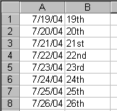
Here’s a formula that I use to get the ordinal day number from a date.
=DAY(A1)&IF(AND(DAY(A1)>=4,DAY(A1)< =20),”th”, CHOOSE(MOD(DAY(A1),10)+1,”th”,”st”,”nd”,”rd”,”th”,”th”,”th”,”th”,”th”,”th”))

There has to be a shorter way than this. What formula do you use?
=DAY(A1) & IF(OR(MOD(DAY(A1)-1,10)>2,INT(DAY(A1)/10)=1),”th”,CHOOSE(MOD(DAY(A1),10),”st”,”nd”,”rd”))
This formula is a tad mathematical but shorter nonetheless.
J-Walk explains this one in a book of his. It doesn’t provide the same result as yours, but seems to work along the same lines.
=TEXT(A1,”mmmm “)&DAY(A1)&IF(INT(MOD(DAY(A1),100)/10)=1, “th”,IF(MOD(DAY(A1),10)=1, “st”,IF(MOD(DAY(A1),10)=2,”nd”,IF(MOD(DAY(A1),10)=3, “rd”,”th”))))&TEXT(A1,”, yyyy”)
Also, suppose you wanted to adapt YOUR formula to show business days, like “7/5/2004? = 3rd (or something like that). In a filldown of a range of dates, weekend days and holidays would come up blank.
Great formula, Dick, et al.
Of course, now we’ll want a macro to apply superscript formatting to the the letters following the number. I messed around with one a couple years ago, and got something passable. Then I just memorized the keyboard shortcuts:
Superscript formatting: Alt+O, Alt+E, Alt+E
Subscript formatting: Alt+O, Alt+E, Alt+B
But I don’t think you could ever do this with a formula resultit would have to be a static value. Or could you?!?
There are really only 7 “special” days, which depend on their last digit. Everything else ends in “th”. Thus:
=IF(ISNA(MATCH(DAY(A1),{1,21,31,2,22,3,23},0)),”th”,INDEX({“st”,”nd”,”rd”},RIGHT(DAY(A1),1)))
Stan
(anal-retentive Stan) — so my last word on this one is:
=INDEX({“st”,”nd”,”rd”,”th”},MIN(RIGHT(DAY(A1),1),4))
Stan – neither of your formulas work. The first one is incorrect at 32. The second one is incorrect as soon as 11.
Andy –
The first one works fine. The 32nd rolls over to the 1st, 2nd, 3rd, or 4th of the next month.
– Jon
Also:
=LOOKUP(MOD(DAY(A1),10)*(INT(DAY(A1)/10)1),{0;1;2;3;4},{“th”;”st”;”nd”;”rd”;”th”})
Daniel M.
There’s a “” between the “10)” and “1?
but the blog parser grabbed it :-(
Hoping it will work this time:
=LOOKUP(MOD(DAY(A1),10)*(INT(DAY(A1)/10) 1),{0;1;2;3;4},{“th”;”st”;”nd”;”rd”;”th”})
Daniel M.
I was looking for a formula to add the ending to a number rather than a date, here is the the formula I used for numbers greater than 0:
=IF(OR(MOD(A1-1,10)>2,MOD(INT(A1/10),10)=1),”th”,INDEX({“st”,”nd”,”rd”},MOD(A1,10)))
Does this work? i’m pretty fluent with advanced formulas but the simplicity of this method is appealing.
=MID(“stndrdthththththththththththththththththstndrdthththththththst”,DAY(TODAY())*2-1,2)
=CHOOSE(MIN(MOD(A1,10)*(MOD(INT(A1/10),10)1)+1,5),”th”,”st”,”nd”,”rd”,”th”)
Handles any number for which you might want such postfixes (that is, positive integers).
=INDEX({“st”;”nd”;”rd”;”th”},MIN(RIGHT(IF(AND(A1>9,A1<14),9,A1)-1)-3,0)+4)
or for numbers past 110
=INDEX({“st”;”nd”;”rd”;”th”},IF(LEFT(RIGHT(0&A1,2))=”1?,4,MIN(RIGHT(A1-1)-3,0)+4))
CHOOSE(MIN(5,MOD(A1,10)*(MOD(INT(A1/10),10)1)+1),”th”,”st”,”nd”,”rd”,”th”)
=CHOOSE(MIN(5,MOD(A1,10)*(MOD(INT(A1/10),10)!=1)+1),”th”,”st”,”nd”,”rd”,”th”)
where != is ‘not equals’
comment form does not permit “
New to VB code, but it was fun and a challenge. This is what I came up with to label a header row based on a week ending date.
Dim DayNumber As String
Dim Ext As String
DayNumber = Day(InputDate)
Select Case DayNumber
Case 1, 21, 31
Ext = “st”
Case 2, 22
Ext = “nd”
Case 3, 23
Ext = “rd”
Case 4, 5, 6, 7, 8, 9, 10, 11, 12, 13, 14, 15, 16, 17, 18, 19, 20, 24, 25, 26, 27, 28, 29, 30
Ext = “th”
End Select
DayEx = DayNumber & Ext
End Function
You can now use it like this…if cell K1=5/3/09
then..
=Dayex($K$1-7) gives you 26th
=Dayex($K$1-6) gives you 27th
=Dayex($K$1-5) gives you 28th
=Dayex($K$1-4) gives you 29th
=Dayex($K$1-3) gives you 30th
@Greg
I get an error with your function
& >;< Ext
Compile Error
Expected End of Statement
For some reason when it was copied and pasted it added the “&”. I no longer have the file because I was using it over a network and it was giving me problems so I just deleted it. But I believe that you can just remove the &
Thanks for trying it out
And for some reason in my reply above its not showing the amp. You have to remove the “& a m p ;” If anyone can explain this I would appreciate it.
=Value&MID(REPLACE(REPT(“thstndrdthththththth”,10),23,6,”ththth”),MOD(Value,100)*2+1,2)
Will work for any value!
=Value&MID(REPLACE(REPT(“thstndrdthththththth”,4),23,6,”ththth”),Value*2+1,2)
If used on dates
Biff (posts under the name T. Valko) and I jointly came up with this formula a couple of years ago or so… we believe it is the shortest formula to place an ordinal suffix on an whole number…
=A1&MID(“thstndrdth”,MIN(9,2*RIGHT(A1)*(MOD(A1-11,100)>2)+1),2)
It may be the shortest, but the one above has less references to change!
While Greg posted his function about a year-and-a-half ago, I thought anyone into VB code might be interested in this one-liner function I’ve posted several times in the past in the compiled VB newsgroups (it works for all numbers, not just date day numbers like Greg’s function)…
Ordinal = Number & Mid$(“thstndrdthththththth”, 1 – 2 * ((Number) Mod 10) * (Abs((Number) Mod 100 – 12) > 1), 2)
End Function
This function was actually the starting point for the formula I posted a few minutes ago.
I also adapted for dates :-
=SUBSTITUTE(TEXT(DateVal,”mmmm dzz, yyyy”),”zz”,MID(REPLACE(REPT(“thstndrdthththththth”,4),23,6,”ththth”),DAY(DateVal)*2+1,2))
this will convert dates into the form “April 23rd, 2010”
“dzz of mmmm yyyy” “23rd of April 2010”
“dddd the dzz of mmmm yyyy” for “Thursday the 1st of April 2010”
“dddd mmmm dzz, yyyy” for “Thursday April 1st, 2010”