Quick Access Toolbar Usage Update

Ever since the great QAT Usage Survey of last year, I’ve had five controls on my QAT. Up from zero. Here’s how they’ve fared.

  1. Borders: Used zero times. I have my two most common border situations (single underline and grand total) available elsewhere. I guess I don’t muck around with borders as much as I thought.
  2. Text to Columns: Used zero times. I use TTC all the time; sometimes one of my own invention, but equally the built-in kind. The built-in kind is good when I have a lot of rows or if I’m tyring to convert a bunch of numbers into text. But I use Alt+A+E without even thinking, so this button has been lonely.
  3. Connections: Used exclusively. Well, kind of. I always start navigating the Ribbon before I remember I have a QAT at all. Then I back out of the Ribbon and Alt+3 to show the external data connections. I think the last couple times I’ve remembered so it’s possible I’ve turned a corner.
  4. Switch Windows: Used zero times. I Ctrl+Tab to switch windows and simply haven’t needed this.
  5. Table Name: Used exclusively. It didn’t take too long to wean myself from Alt+JT+A to Alt+5. This has been the biggest success.

The QAT has awesome Alt+n shortcuts that I need to use. I just don’t know what to put on there. I use Borders and Switch Windows far less than I thought. I need to find some that I’ll actually use.

First bug of the year

And it’s a funny one. Save all your work, then make up a simple datasource that has a formula in the header:

 
SomeFormula
 
 
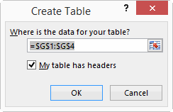
Now, turn the Macro Recorder on, and while it’s recording, turn that datasource into an Excel Table. (I use the Ctrl T shortcut for that)
 
Create Table
 
 
Excel will warn you that the formula will be converted to static values. Click No.
 
Continue
 
 
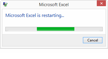
Beeeeep.
 
Restarting

Happens for me using Office 365. Pretty obscure, granted.

What Is the Most Awesome Microsoft Product

As if you didn’t know.

As the people talked, we started to get a sense for why they thought Excel is cool – Excel enables people to be rockstars at their jobs and get recognition from their peers. Excel makes people feel powerful. Excel is a work tool that people *love* to use.

You can also read the rest of the answers. Lots of OneNote and Kinnect. Even a Visio and a Minesweeper.

Evaluate Mid

In my last post, I created an array from formula text by using VBA’s Evaluate method, in order to roll my own FormulaArray function that displays the array returned by a formula, for documentation purposes.

In the course of this, I’ve discovered something a bit weird about how this method evaluates the arrays returned by a MID function.
Let’s use this snippet:

Sub EvaluateThis()
Dim var As Variant
var = ActiveSheet.Evaluate(ActiveCell.Formula)
End Sub

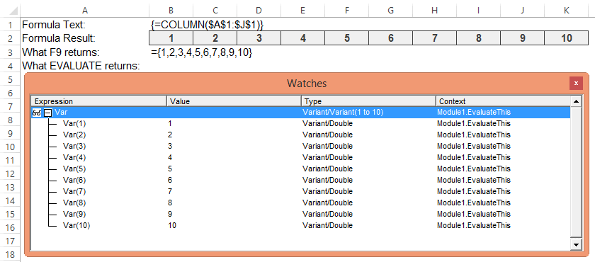
First, let’s look at how it handles an array generated by the COLUMN() function:
 
Evaluate COLUMN array2


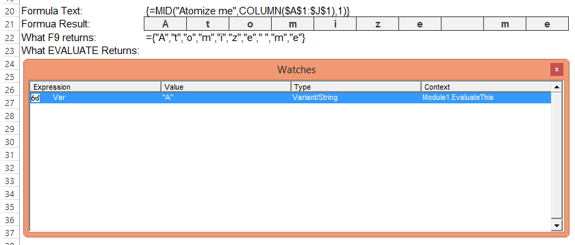
Now watch what happens when we use that array to split apart a string using the MID() function:
 
Evaluate MID array2


So if you push F9, you get an array, but if you use the Evaluate method you don’t…you just get the first letter. Is this weird, or am I missing the point?

Evaluate(Evaluate)

Since Excel 2013, Microsoft has given us a FORMULATEXT function, which if you point at a cell will do just that. Here’s a naughty snapshot of FORMULATEXT playing with itself in the corner:
 

FormulaText
 
 
I thought I’d have a go at writing a FormulaArray function to complement it, because when I’m building up a complicated formula that uses lots of array manipulation, then I like to document how all the different arrays within it fit together. (I was going to say “come together” there, but after that crack about FORMULATEXT playing with itself, I thought better of it. But now that I’ve said crack, I’m gonna throw caution to the wind and say wind too.)

Currently I document my formula beasts by either either array-enter a sub-part in the sheet with some notes, like this:
 
Documentation 1
 
 
…which shows how my ExtractNumber formula works, or I enter the desired formula in one cell with a ShowFormula to the left and a hand-rolled hard-coded array to the right, like in this table where I’m documenting a few ways to dynamically generate consecutive integers:
 
Documentation 2
 
 
I get that ResultArray manually, by clicking in the formula bar, pushing F9, copying the resulting evaluated array, then pasting it in another cell. Tedious. Especially when I later make a change to that sub-part, because then I get to do those steps all over.

So I started to roll my own FormulaArray function. I got a bit bogged down in the joining bit, but after about an hour of Googling, I rediscovered Nigel Heffernan’s code for joining two dimensional arrays. Which is very concerning, because I discovered it like just 10 days ago, and even wrote an extensive blog post on it right here. Senility is obviously setting in. If I start saying the same thing over and over like my mother does, just shoot me. If I start saying the same thing over and over like my mother does, just shoot me.

Anyways, Nigel’s function needs a 2D array. You can create an array from formula text by using VBA’s Evaluate method. If the formula returns a Row vector or a 2D vector, then Evaluate nicely turns it into a 2D vector. But here’s the rub: if the formula returns a Column vector, then Evaluate only gives us a 1D vector, which ain’t gonna wash with Nigel’s function:
 
Row vs Column
 
 
So what we need to do is TRANSPOSE any formulas that would return Column vectors, because chucking a TRANSPOSE into the mix has the desired effect:
 
Row vs Column2
 
 
Note that I’m using the square brackets [ ] shortcut for Evaluate. I could just have easily done it like this:
 
Row vs Column3


Okay, so we know that if our formula string returns a Column vector, we’ve got to transpose it. But how can we tell that ahead of time? I can’t think of a way. So I just do this:


Function FormulaArray(Target As Range) As String
Dim strInput As String
Dim var2 As Variant
Dim lb As Long

strInput = Mid$(Target.Formula, 2)
var2 = ActiveSheet.Evaluate(strInput)
On Error Resume Next
lb = LBound(var2, 2)
If Err.Number <> 0 Then
var2 = Application.Transpose(ActiveSheet.Evaluate(strInput))
FormulaArray = Join2d(var2, ",", ";")
Else:
FormulaArray = Join2d(var2, ";", ",")
End If

End Function

So I evaluate the formula as if it’s a Row vector, then check if I’ve got 2 dimensions as a result. If not, it must have been a column vector, in which case I transpose it, then reevaluate it. Shame about the double evaluation, but I can’t think of a foolproof way to do it differenty, other than perhaps array entering the formula into a 2D range on the worksheet and looking at where the #N/A! errors fall.

Anyway, it seems to work just fine:
 
Result_NoTable2


..unless you happen to be using Structured Table References, and your arguments happen to use the @ table notation to point at something on the same row:
 
Result_SameTable
 
 
…or unless you happen to have a formula with the INDIRECT function in it:
 
Result_INDIRECT2
 
 
With the ThisTableRow thing, I guess I can just replace the @[SomeColumn] bit with the actual address, but I can’t think of easy ways around the INDIRECT thing. Anyone got any ideas?

Edit: Thinking about this some more, all I need to do is substitute the INDIRECT(SomeExpression) with whatever gets returned by RANGE(SomeExpression).value

Sample workbook:

FormulaArray_20141125

There’s a handy post over at Charles Williams’ site that talks about some other quirks of Evaluate that’s worth checking out:
https://fastexcel.wordpress.com/2011/11/02/evaluate-functions-and-formulas-fun-how-to-make-excels-evaluate-method-twice-as-fast/

Out, damn’d gridlines! Out, I say!

So after doing some incredibly complicated formula challenges and ninja-grade VBA, I thought I’d turn my hand to something simple: finally changing the default template that loads when Excel starts or when I create a new workbook or worksheet so that gridlines are turned off. Because if there’s one thing I hate about Excel, it’s those gridlines: they make everything look like it was done in Excel. And if there’s one thing I do as soon as I open a new file, it’s turn those gridlines off. Tables and PivotTables give me all the borders I need, thank you very much.

Boy, what a battle. I have saved my changed book as an XLTM to just about everywhere I can think of.

  • I’ve tried saving it to C:\Users\Samsung\AppData\Roaming\Microsoft\Excel\XLSTART but when I start Excel, I have gridlines.
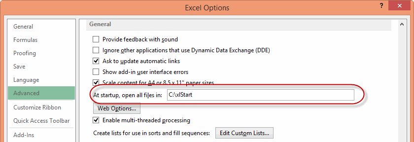
  • I’ve tried creating a new file at C:\xlStart with the template in it, and told Excel via Options>Advanced to open files in that folder but when I start Excel, I have gridlines:

    Options

  • I’ve saved it to C:\Users\Samsung\Documents\Custom Office Templates but when I start Excel, I have gridlines

I’ve gone from feeling like I’ve mastered to Excel, to feeling like I’m a complete idiot. Anyone care to tell me that I’m not?

How the heck the average user is supposed to know how to do this stuff is beyond me. Why isn’t there simply a button on the ribbon or backstage that says:
Give all future workbooks the settings of this one.

I’m using Excel 2013 365. But I’m thinking of doing a complete 180.

Dynamically extracting the nth numerical element without delimiters

ExcelXOR has a great post on using formulas to extract all numbers from a string where:

  • The string in question consists of a mixture of numbers, letters and special characters
  • The numbers may appear anywhere within that string
  • Decimals within the string are to be returned as such
  • The desired result is to have all numbers returned to separate cells

That’s a tall order with formulas. Here’s what ExcelXOR came up with:


=0+MID(“α”&s&”α0″,1+SMALL(IF(MMULT(0+(ABS(51.5-CODE(MID(SUBSTITUTE(“α”&s&”α0″,”/”,”α”),ROW(INDIRECT(“1:”&LEN(“α”&s&”α0″)-1))
+{0,1},1)))>6)*{2,1},{1;1})=2,ROW(INDIRECT(“1:”&LEN(“α”&s&”α0″)-1))),e),SUM(SMALL(IF(ISNUMBER(MATCH(MMULT(0+(ABS(51.5-CODE(
MID(SUBSTITUTE(“α”&s&”α0″,”/”,”α”),ROW(INDIRECT(“1:”&LEN(“α”&s&”α0″)-1))+{0,1},1)))>6)*{2,1},{1;1}),{1,2},0)),ROW(INDIRECT(
“1:”&LEN(“α”&s&”α0″)-1))),2*e+{-1,0})*{-1,1}))

…where s is the string you want to break apart, and e the element you want returned.

That fatboy runs to 415 characters. Which is a heck of a lot less than my first effort:

=SUM(IFERROR(--REPT(MID(s&"|",ROW(OFFSET($A$1,,,LEN(s)))*COLUMN(OFFSET($A$1,,,,LEN(s)))^0,COLUMN(OFFSET($A$1,,,,LEN(s)))*ROW(
OFFSET($A$1,,,LEN(s)))^0),(IF((ISNUMBER(-MID(s&"|",ROW(OFFSET($A$1,,,LEN(s)))*COLUMN(OFFSET($A$1,,,,LEN(s)))^0,COLUMN(OFFSET(
$A$1,,,,LEN(s)))*ROW(OFFSET($A$1,,,LEN(s)))^0))*NOT(ISNUMBER(-MID("|"&s&"|",ROW(OFFSET($A$1,,,LEN(s)))*COLUMN(OFFSET($A$1,,,,
LEN(s)))^0,COLUMN(OFFSET($A$1,,,,LEN(s)))*ROW(OFFSET($A$1,,,LEN(s)))^0)))*NOT(ISNUMBER(-MID(s&"|",1+ROW(OFFSET($A$1,,,LEN(s)))
*COLUMN(OFFSET($A$1,,,,LEN(s)))^0,COLUMN(OFFSET($A$1,,,,LEN(s)))*ROW(OFFSET($A$1,,,LEN(s)))^0))))>0,ROW(OFFSET($A$1,,,LEN(s)))
*COLUMN(OFFSET($A$1,,,,LEN(s)))^0) = SMALL(IF((ISNUMBER(-MID(s&"|",ROW(OFFSET($A$1,,,LEN(s)))*COLUMN(OFFSET($A$1,,,,LEN(s)))^0,
COLUMN(OFFSET($A$1,,,,LEN(s)))*ROW(OFFSET($A$1,,,LEN(s)))^0))*NOT(ISNUMBER(-MID("|"&s&"|",ROW(OFFSET($A$1,,,LEN(s)))*COLUMN(
OFFSET($A$1,,,,LEN(s)))^0,COLUMN(OFFSET($A$1,,,,LEN(s)))*ROW(OFFSET($A$1,,,LEN(s)))^0)))*NOT(ISNUMBER(-MID(s&"|",1+ROW(OFFSET
($A$1,,,LEN(s)))*COLUMN(OFFSET($A$1,,,,LEN(s)))^0,COLUMN(OFFSET($A$1,,,,LEN(s)))*ROW(OFFSET($A$1,,,LEN(s)))^0))))>0,ROW(OFFSET
($A$1,,,LEN(s)))*COLUMN(OFFSET($A$1,,,,LEN(s)))^0),e))),0))

…although there is some pretty nifty stuff going on in there, that I’ll bore you with at a later date…including a MID that breaks a string down into ALL possible slices of text:
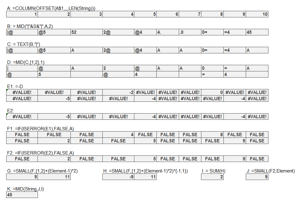
=MID(s&"|",ROW(OFFSET($A$1,,,LEN(s)))*COLUMN(OFFSET($A$1,,,,LEN(s)))^0,COLUMN(OFFSET($A$1,,,,LEN(s)))*ROW(OFFSET($A$1,,,LEN(s)))^0)

I couldn’t rest with just that. Literally. It was too heavy. So I had another crack. The result: Here’s a generic ExtractNumbers formula I just put together. And by ‘just’ I mean I only just managed it, and it took an entire weekend, I ignored the kids, and forgot to bathe. (That last one is pretty much a given, and I can’t really blame Excel).


=MID(s,SMALL( IF( ISERROR( -MID( TEXT( MID("||"&s,ROW( OFFSET( $A$1,,,LEN( s))),2),"|"),2,1)),FALSE,ROW( OFFSET( $A$1,,,LEN( s)))),e)
-1,SUM( SMALL(IF( ISERROR( -MID( TEXT( MID("|"&s&"|",ROW( OFFSET( $A$1,,,LEN( s)+1)),2),"|"),{1,2},1)),FALSE,ROW( OFFSET( $A$1,,,LEN(
s)+1))),{1,2}+(e-1)*2)*{-1,1}))

…again, where:
S = the string you want to break apart
E = the number element you want to return

It will handle numbers with decimal places provided there is a digit to the left of the decimal place e.g. SomeText5.745 and NOT SomeText.745, and it’s a much more svelte 277 characters in length. Isn’t she a beauty? A lot of the inspiration for the approach came from Excel Ninja Sajan, over at the awesome Formula Challenges section of Chandoo’s forum.

In that incarnation, you can use it to extract just one element of a specific number:
 
Extract1


Or if you prefer, you can use this version:
=MID($A28,SMALL(IF(ISERROR(-MID(TEXT(MID(“||”&$A28,ROW(OFFSET($A$1,,,LEN($A28))),2),”|”),2,1)),FALSE,ROW(OFFSET($A$1,,,LEN
($A28)))),COLUMNS($B28:B28))-1,SUM(SMALL(IF(ISERROR(-MID(TEXT(MID(“|”&$A28&”|”,ROW(OFFSET($A$1,,,LEN($A28)+1)),2),”|”),{1,2},1)),
FALSE,ROW(OFFSET($A$1,,,LEN($A28)+1))),{1,2}+(COLUMNS($B28:B28)-1)*2)*{-1,1}))

…you can use it to extract numbers into separate columns, where $A28 holds the string to be split, and B28 holds the first column that you want to extract a number to. Like so:
 
Extract2


I don’t know how either of these perform against a UDF, let alone each other. Anyone got a lean, mean, UDF-based splitting machine that we can test it against?

Here’s a sample file:
ExtractNumber_20141120

—Edit 21 Nov 2014—
It turns out that my above formula fails for a few specific special character & number combinations. Here’s a table, showing in which cases Excel will still treat a number as a number when you pad it out with a non number. For completeness I do three tests:

  • Special character before the number
  • Special character after the number
  • Special character on either side of the number

 
special character matches

—Edit 8 Dec 2014—
Crikey…after chaining myself to the computer since the last update, I finally managed to cobble together a formula that will extract all numbers in practically any shape or form that the local version of Excel deems as a number. That is, given a string like this:
Jeff Weir Age: 43 DOB: 25/4/71 Salary: $100,000 StartTime: 8:30
…It returns this
43
25/4/71
100000
8:30

It ain’t pretty. If you like UDFs, then you’ll agree with my pal Gareth Hayter that this is pure formulabation. Unless you like formulas, in which case it’s orgasmic. (You sick, sick analyst, you. Don’t let your boss catch you playing with it in the office…)


=MID( String,SMALL( IF( ( FREQUENCY( ISNUMBER( -MID( String,ROW( OFFSET( $A$1,,,LEN( String)))*COLUMN( OFFSET( $A$1,,,,LEN( String)))^0,COLUMN( OFFSET( $A$1,,,,LEN( String)))*ROW( OFFSET( $A$1,,,LEN( String)))^0))*( COLUMN( OFFSET( $A$1,,,,LEN( String)))+ROW( OFFSET( $A$1,,,LEN( String)))-1),ROW( OFFSET( $A$1,,,LEN( String)+1))-1)=1)*ISNUMBER( -MID( "|"&String&"|",ROW( OFFSET( $A$1,,,LEN( String)+2)),1))=1,ROW( OFFSET( $A$1,,,LEN( String)+2))-1,FALSE),ROW( OFFSET( $A$1,,,LEN( String)))),SMALL( IF( ( FREQUENCY( ISNUMBER( -MID( String&"|",ROW( OFFSET( $A$1,,,LEN( String)))*COLUMN( OFFSET( $A$1,,,,LEN( String)))^0,COLUMN( OFFSET( $A$1,,,,LEN( String)))*ROW( OFFSET( $A$1,,,LEN( String)))^0))*( LEN( String)+1-ROW( OFFSET( $A$1,,,LEN( String)))),MOD( LEN( String)+2-ROW( OFFSET( $A$1,,,LEN( String)+1)),LEN( String)+1))=1)*ISNUMBER( -MID( "|"&String,ROW( OFFSET( $A$1,,,LEN( String)+2)),1))=1,ROW( OFFSET( $A$1,,,LEN( String)+2))-1,FALSE),ROW( OFFSET( $A$1,,,LEN( String))))-SMALL( IF( ( FREQUENCY( ISNUMBER( -MID( String,ROW( OFFSET( $A$1,,,LEN( String)))*COLUMN( OFFSET( $A$1,,,,LEN( String)))^0,COLUMN( OFFSET( $A$1,,,,LEN( String)))*ROW( OFFSET( $A$1,,,LEN( String)))^0))*( COLUMN( OFFSET( $A$1,,,,LEN( String)))+ROW( OFFSET( $A$1,,,LEN( String)))-1),ROW( OFFSET( $A$1,,,LEN( String)+1))-1)=1)*ISNUMBER( -MID( "|"&String&"|",ROW( OFFSET( $A$1,,,LEN( String)+2)),1))=1,ROW( OFFSET( $A$1,,,LEN( String)+2))-1,FALSE),ROW( OFFSET( $A$1,,,LEN( String))))+1)

Here’ a file showing how this bit of formulabation comes together: Dynamic Split Numbers_20141208 v6

An INDEX of insights from ExcelXOR

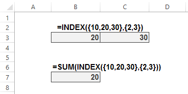
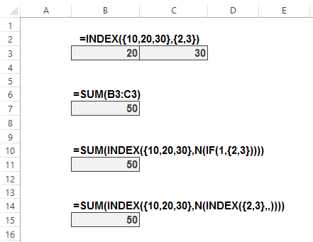
Everybody knows that you can’t do some things with the result of an INDEX function unless you return it to the worksheet first. For instance, I can return the 2nd and 3rd members of the array {10,20,30} to the worksheet with an array-entered INDEX function like this:
 

Index1
 
 
…but if I wrap a SUM around that INDEX and array enter it, I get the wrong answer:
 
Index2
 
 
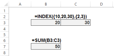
…meaning I have to return that INDEX function to the grid and then point my SUM function at it:
 
Index3
 
 
Everybody knows that, right? Well, everybody’s wrong. Everybody but the author over at the new ExcelXOR blog, that is. At this earth-shattering post the Author shows several intriguing ways to get INDEX to play nicely with outer functions:
 

Index4


Far out! That’s the kind of trick I would have sold my soul to the devil to learn.

There’s a lot to learn at that site: go to http://excelxor.com/blog/ and scroll most of the way down until the Archives section, and then get clicking. The earliest post is practically from yesterday: August 2014. But there’s a lifetime of learnings there already…both in the posts, and in the comments. Plus the most wicked formula challenges you will find in one place.