Well THAT sure got your attention.

I was doing a bit of research for the book (the only bit, mind), and I came across this great old thread on VLOOKUP vs INDEX/MATCH.

There’s a few false starts in terms of test methodology until Jon von der Hayden puts things back on the right track about halfway through the thread.

Conclusion is that INDEX/MATCH is probably way to go, but there’s not a great deal in it.

But I think there’s another important point in the INDEX/MATCH combo’s favor that has been overlooked in this thread: and that’s this bit in bold:

=VLOOKUP(lookup_value,table_array,col_index_num,range_lookup)

The fact that a VLOOKUP functions points at an entire table of data – even though it only ever actually makes use of two columns of it (the key column on the far left, and the nth column given by the col_index_num argument) – means that any time you change any cell in that table, your VLOOKUP is going to recalculate. And then so are ALL formulas downstream of those VLOOKUPS. It’s exactly as if VLOOKUP is a volatile function, where changes to that that Table is concerned.

Whereas with INDEX/MATCH, your functions will ONLY recalculate if you change something in the specific columns that the INDEX and MATCH combo references.

Given that, I’ll take INDEX/MATCH any time.

One thing still puzzles me hugely about VLOOKUP though: the recalculation time incurred from updating the lookup table seems much much longer than the recalculation time incurred from changing an input parameter for the VLOOKUP itself. And the same goes with INDEX/MATCH.

Take the situation where you’ve got a VLOOKUP and Table that looks like this:
 

 
 

The KEY column is just the numbers 2 through 1,048,576 sorted in random order. And the Value column is just the row number. I won’t post a sample file because it runs to about 20MB, but it’s easy to set up yourself in about 20 seconds.

Changing the orange input cell triggers the VLOOKUP, which gets the right answer pretty quick. I haven’t timed it, but we’re talking ‘blink of an eye’… even when I tell it to look for a number that I happen to know is right at the bottom. Really fast.

But if I type anything in that middle column in the Table – which also causes our VLOOKUP to recalc – Excel acts really really sluggish. Maybe a second of delay in some cases, plus it makes my screen flash.

Which is weird, because it’s the same one VLOOKUP that gets triggered in both cases.

Why would that be?

—UPDATE—
If you haven’t already, go and read Charles Williams’ awesome article Developing Faster Lookups – Part 1 – Using Excel’s functions efficiently – updated

Look for the bit “Large dependency ranges trigger unnecessary Lookups”.

Read it, and don’t weep.

I’m getting close to finishing off the first draft of my book, and I’m putting some goofy images at the start of every major section, to lighten it up. I want this to be a laugh-out-loud Excel book: my goal with these images is to make some schmuck reading an Excel book snort out loud on the train during their commute, so that fellow commuters figure this is one sad individual.

In fact, I’m hoping more people will buy it “just for the pictures”, like my mother has promised to. Which is why I put an attractive picture of my wife and I on the cover:

So anyways, while I was putting some sample images and text together – all the while snorting out loud to myself at the endless possibilities for entertainment that random animal pictures combined with Excel witticisms provide – I thought why not get you lot in on some of the fun as well. And so I’ve cooked up a grand scheme: the great “Your Name Here” competition.

So here’s the deal: below are some of the sample images I’ve put together so far, using comp images I’ve downloaded from iStock. (I’m sure that my publisher Bill Jelen is going to choke on his morning podcast when he sees I’m serious about some of these).

Your mission – should you choose not to simply laugh it off – is to improve on these in some way if you dare. (I was going to say if you can, but I can tell by your face that you have innate comic ability).

By ‘improve on these in some way’, you’ve got two options:

1. Come up with a better caption with your name in it; or
2. Come up with a better image a better caption with your name in it.

Prize? Oh yeah…hmmm…okay, let me think. How about you get to win a copy of my as yet unfinished book. With that winning picture in it. And caption. With your name in the caption. Just your first name, mind, given that tens, possibly twenties of people will see your name next to some random monkey picture or whatever, and wonder what it means in terms of your Excel prowess. Can’t drag your good name down with mine, can we….

Couple of rules:

 
1. Entries close at the end of this Month (March 2015), and I’ll endeavor to review submissions and get back with some winners and honorable mentions within a fortnight after that.

 

2. If you just want to just submit a caption, don’t email it to me, but instead simply put it below in the comments along with the heading number and name its’ associated with, so we can all share your mirth right away. (You don’t have to put your email address in the comment, because this blog keeps track of your email when you post a comment, so I’ll be able to contact you if you have a winning entry).

 

3. If you want to provide a different image than the ones below as well as a caption, feel free. But please ether use a free image from WikiMedia and include the link in your submission, or a free comp image from iStockPhoto, again with the link. And I need an aspect ratio along the lines of these ones i.e. wider than they are tall like the samples below, so they will fit where I plan to put them in the book, and so that I can purchase the image if it’s going to be used.

   Also, if providing an image, make sure it’s of an animal – the wilder the better – so that it fits with the general theme of the other pictures I’ll be using in the book.

 

Images 6 and 11 below come from Wikimedia. Simply Google WikiMedia and some animal name to see what’s available there. Here’s an example, that shows a Monkey taking a selfie. (I kid you not):

The rest came from iStock. What’s iStock, and what’s a comp image? Just head to www.iStockPhoto.com, type something like ‘Animals’ or what-not in the big search box on the home page, and when you get to the search page, refine it further by unchecking illustrations, video, and audio options:

Then when you see something you want to use, click on it, which will bring it up bigger:

Then you can either click that ‘Get a comp’ option and copy the image that comes up, or simply right click the image shown above and select ‘Copy as Image’ and then paste it into this template and add a caption:
Competition Template

Then simply email it to me at excelforsuperheroes@gmail.com

Have fun, people.

Here’s my sample images, with placeholder text/names. But first, a disclaimer

Disclaimer

All physical characteristics appearing in this work are fictitious. Any resemblance to real MVPs, past or future, is purely coincidental.

1. Chris

2. Rob

3. Ken

4. Jeff

5. Jon

6. Doug

7. Ian

8. Deb

9. Dick

10. Mike

11. Charles

12.Oz

13. Mynda

14. Dave

Even though you’ve seen Excel’s Formula Intellisense a million times, I bet there’s a few things that you don’t know about it that can make your life even easier.

Let’s first look at an example for one of Excel’s in-built functions. Say we want to use an IFERROR function. As soon as we type the = sign in the toolbar and the opening ‘I’ from IFERROR, Excel provides a helpful list of functions that start with the letter ‘I’, as well as a pop-up tool tip telling us what the currently highlighted function from that list does. That popup tool tip is often in the way, but you can move it somewhere else simply by clicking on it and dragging it to the naughty corner.
 

 
 
To select the IFERROR function from that list, we can either use the arrow keys to navigate down that intellisense list, or we can left-click on the particular function we want:
 

 
 
…or we can continue typing, which allows Excel to gradually narrow down the number of functions until there is only one possible choice…the IFERROR function we’re after:
 

 
 
At this stage, I almost always push Enter in order to get Excel to populate this one remaining function in the intellisense list into the formula bar. And then I almost always swear out loud, because Enter is the incorrect key, and because Excel has never heard of an ife function, it asks me for my name, so that it can pass it on to the ‘re-education’ team at Microsoft:
 

 
 
The correct key we need to push is the TAB key, which tells Excel to fill out the rest of the IFERROR name for us. After it’s done this, Excel then helpfully prompts us for the two arguments of the IFERROR function with another handy pop-up tool-tip:
 

 
 
Now let’s compare that to the options Excel gives us for a UDF. I’ll use my JoinText UDF. Typing =j pops up a very short list indeed: there are no other functions starting with J. But the UDF’s name is all we get. There’s no tooltip remindingus what the JoinText function actually does…
 

 
 
…and after we select it by hitting that TAB key, there’s no tooltip prompting us for the function arguments:
 

 
 
So why don’t UDFs have intellisense? That’s a damn good question, and one that programmers have been asking Microsoft about for years. If you can’t remember the arguments for your UDF, you won’t be getting very far. Unless you happen to know this handy little trick: If you push CTRL + SHIFT + A at this stage, Excel helpfully inserts placeholders for all the argument names for that function into the formula bar:
 

 
 
…which you can then overtype with the actual arguments, now that you’ve been reminded what they are. How cool is that!

This trick also works with Excel’s native functions, too:
 

 
 
But the problem we still have with that UDF is this: Which arguments are optional? In the case of the VLOOKUP above, we can see this by the square brackets around the optional [range_lookup] argument in the tool-tip. (As if that argument is optional in the real world…)

But with our UDF, we don’t get that tool-tip pop-up.

Sure, we could just put the prefix opt in front of the optional arguments in the VBE:
 

 
 
…which would give us this:
 

 
…but where’s the fun in that?

It would be cool if we could simply add square brackets to our variable names back in the VBE, so that when we do our Ctrl + Shift + A trick, those arguments look like this:
 

 
 

…but it won’t compile:
 

 
 

So what other interesting characters can we use in VBA variable names? According to this thread, these ones:
 

 
 
Any character in the range 128-255 is allowable. That’s right, you can copy-write and trademark your variable names if you want!

And a couple of them look quite bracketish. Let’s try them:
 

 
 
Yup, that compiles. And how does it look when we Ctrl + Shift + A that sucker?
 

 
 
Hmmm. Works a treat.

Down side? Don’t know. You tell me…

A couple of days ago I floated the concept of a dedicated annual “Still Broken” week in which we can talk very honestly about the things in this otherwise great application that we think are still broken, plus review our list from the same time last year to see if any action has been taken by our gracious host…that would be Microsoft…to actually remedy anything we were bitching about the previous year. And just as importantly, to give credit where credit is due…because let’s face it…it’s not trivial to make changes to something that 750 million odd users are using at the time.

100% of the comments of that post that directly mentioned this concept were generally supportive (thanks, Doug). So I thought “There’s no week like the present”.

And so, without further ado, here’s a bit of Excel that I was playing with today that strikes me as being not quite finished: the Add-ins options.

Why is it that if I save a brand new Add-in to the Add-ins folder:
 

 
 
…it doesn’t automatically show up in this window, under the Inactive Application Add-ins section?
 

 
 
…and yet if I click the Go button next to Manage Excel Add-ins, I see that Excel obviously knows about it: Edit: And even though I parked it in the right car-park building, it still won’t show up until I politely point Excel to the exact spot I parked it in:
 

 

 

 
 
Given it was correctly stored in the Add-ins folder, why didn’t you just let me automatically populate it into the ‘Inactive Application Add-ins’ part of the Excel Options/Add-ins pane like this from the get go:
 

 
 
…and then let me decide to activate it just by double clicking on that listing?

Currently, selecting an Add-in from that Excel Options dialog and double clicking does absolutely nothing. What’s the point in letting me even select it…it’s not like I can actually do anything with it. All you’re doing is giving me vain hope.
 

 
 
Furthermore, jumping back a few steps now, whenever I push OK from that Add-ins dialog box:
 

 
 
…why do you automatically assume I’m done with the Excel Options dialog box I came from, and close it? Is it inconceivable that I might want to manage more than one Add-in? Or that my intention was to manage a COM add-in, but I forgot to change that default Excel Add-ins option in the dropdown, and want some simple way to go back and choose the other option? Sheesh.

Please Microsoft…don’t make me click. Here’s a thought: hire someone to the newly created position of “Manager, Click Reduction”, and empower them to champion basic design changes that let users use your interface much more efficiently. I’m available.

In fact, I think you need to take an honest look at what you expect users to do in order for them to leverage off of Add-ins. I think the current system presents too much of a barrier to non-technical people who would otherwise be able to make much more out of your fine application. I’ve just spent quite a few days writing the chapter in my book that explains how users can leverage off of Add-ins without having to have one jolt of knowledge of VBA. Unfortunately, my conclusion is that while they don’t have to be VBA experts, they do have to be “Install an Add-in” experts, because the process is not as simple and genius as it could be.

Okay, that’s kick-started the week. Who’s up next. Anyone? Anyone?

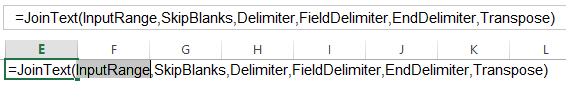
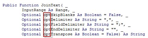
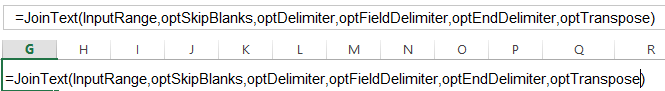
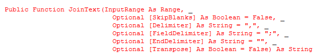
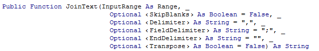
I like Colin Legg’s cool code over at Self Extending UDFs – Part 1 and Self Extending UDFs – Part 2. And I keenly await Self Extending UDFs – Part 3 (subtitled Return of the User-i or something similar)

If you haven’t seen those articles, go check ’em out…they show you how you can use a UDF to change something on the worksheet. Particularly handy where you have array formulas that you can’t be arsed resizing. (And before y’all start yelling Nooooooooooo… at me, I’m going to yell back preemptively: As Colin points out, if it’s good enough for Google Sheets to offer this kind of thing via their UNIQUE and SORT functions, it’s good enough for Microsoft Excel too. Microsoft ALREADY lets the user overwrite data accidentally anyhow, with things like the Advanced Filter, etc. What’s so sacred about UDFs?)

What I’d like to see next along these lines is something similar to this concept where you can have a UDF called RunMacro(Target, Macro, [Condition]) that would let non VBA programmers run point-and-click macros and functions when something on the sheet changes. Sure, you and I would just set up an event handler. But I think ‘normal’ users should be able to set up event handlers too. Why not via a UDF? And so I wonder if Colin’s code can be amended to do this? (I haven’t delved into your code yet)

Here’s a hypothetical situation where I think such a function would be useful: filtering PivotTables based on an external range. I wrote a function here sometime back who’s arguments are a range where a PivotField is, and a range where a list of filter terms is. It looks something like this:
Private Function FilterPivot(rngPivotField As Range, rngFilterItems As Range) As Boolean

Imagine if you could call that right from a UDF in the worksheet, so that a user could dynamically filter a Pivot – or an entire Pivot-based dashboard – simply by pasting new data into the rngFilterItems. Much handier than having to manually click a slicer.

Sure, you can write an event-handler to do this…if you know how to write an event handler. Why not give this type of functionality to the average programmer, too? Let me remind you that the average programmer programs Excel with Formulas, and may not know their VBA For from their Next. But that doesn’t mean they shouldn’t be able to trigger well-thought-out macros directly from the sheet, surely?

Which reminds me of Oz Du Soleil’s latest post Google Has Gone Mad, which is a great post. In fact, I love all of Oz’s posts as much as I like his hat collection and his cool surname. (Mine is just “Weird” without the “d”). So should you, so go and subscribe to his blog now if you’ve never heard of the man. And check him and the team out at Excel.tv.

Oz makes the point that it’ll take a much longer time for an Excel user to need to resort to VBA compared to an “enlightened” Google Sheets user who’ll need to be good at JavaScript to do anything remotely as interesting as you can do in Excel. And in typically beautiful turn of phrase, he puts it like this:

Let’s present this at the most extreme. Pick one:

Pay the nanny state [Microsoft] or
Live in the open wilderness [Google Sheets]

Neither is bad, but you need to have a sober assessment of what you’ll need to live in the wilderness before you freeze to death under an unvalidated spreadsheet.

Man, I wish this guy was writing my book instead of me.

But while I agree with that, I think it’s our duty to constantly remind the Nanny State that there is still a LOT of unfulfilled potential in this here ‘virtual country’ that we all share. Yes, we voted for them with our wallets…but largely because the other guy’s policies looked far worse for the economy. In fact, sometimes we get irked because we see a lot of fluffy stuff that looks like it’s more focused on attracting votes than improving outcomes, and meanwhile some old irritants are now very old indeed. Some are over a decade old now.

That’s actually a key point of the book I’m supposed to be writing right now instead of this blog post. It’s called Excel for Superheroes and Evil Geniuses: An irreverent guide to getting Microsoft Excel to do your dirty work. A superhero is someone who uses the right bit of the application to do something as efficiently as it can be done out of the box. So they happily live in the Nanny State’s protection, and thanks to their advanced knowledge, they live well. Whereas an Evil Genius is someone who has a powerful arsenal of ‘borrowed’ technology at their disposal in the form of some killer User Interface tweaks, User Defined Functions, and weapons-grade Add-ins. They might not actually understand one single line of VBA code, but that doesn’t stop them from using incredibly powerful point-and-click Macros to pimp Excel so that it runs faster, meaner, and leaner than even a Superhero could make it run.

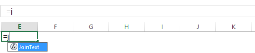
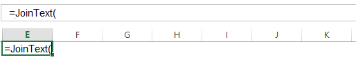
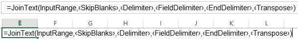
Of course, the Evil Geniuses of my book only need code because the Excel UI holds even Superheros back due to some poor choices in UI design. For instance, out of the box, you can’t filter a PivotTable on an external list automatically. You don’t have a viable dynamic concatenate function. You can’t natively deselect something in your selection, without wiping your entire selection. You can’t see long references in the Go To box because it ain’t wide enough, and it doesn’t let you resize it. And many, many, many more things that to me seem like easy-to-improve no-brainers.

I guess we’ve got to keep voting for the Nanny State, but that doesn’t mean we can’t tell them that we shouldn’t have to become Evil Geniuses just to fix suboptimal stuff in their “country”. And we should definitely point out to the Nanny State that we like – no, love – the look of some of the ‘policies’ of the other party. Even if the other party is not a credible threat, come election time (or 365 subscription renewal time, rather). Even if on balance, deep down inside we really love the Nanny State and would never renounce our citizenship.

Despite the fact that they don’t seem to listen, I think we simply have to keep loudly demonstrating on these virtual streets about things that should be a fundamental right to every citizen that lives here. Can’t filter a PivotTable on an external list natively? Tell the Nanny State. Still don’t have a viable concatenate function after all these years? Tell the Nanny State. No way to natively deselect something in your selection, without wiping your entire selection? Tell the Nanny State. Can’t see long references in the Go To box because it ain’t wide enough? Tell the Nanny State. And keep telling them. Don’t let up. Even if you’re just shouting it into the cyber wind, as I am here.

Of course, the Nanny State has to balance what they believe is best ‘on balance’ for the entire country against what they will think will keep them in power. And of course, they’re always going to be doing some stuff that’s more focused on attracting marginal voters in swing states than you and I in the beltway. Which means they’re probably unlikely to prioritize what I consider to be some simple no-brainers that we’ve been asking for for ages. Which also means we have to use a UI which is good enough so that users don’t absolutely have to learn VBA to do stuff, but in many cases is FAR from optimal. Far from perfect.

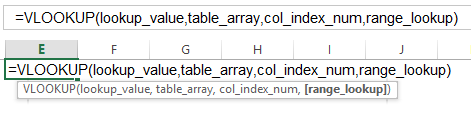
Shouting into the cyber wind by yourself can seem pretty pointless though. Which is why I’ve had an idea. We’ve had VLOOKUP week, and we’ve had some other similar week that Chandoo kicked off recently (but the theme of which eludes me right now). How about a dedicated annual “Still Broken” week in which ALL of us that can talk very honestly about the things that we think are still broken, plus review our list from the same time last year to see if any action has been taken by the Nanny State to actually remedy anything we were bitching about back then. And then give credit where credit is due…because let’s face it…it’s not trivial to make changes to something that 750 million odd users are using at the time.

Anyways…about that week. Here’s my ideas for names:

• “The week of tough love.”
• “Vote with your bleat” (Very fitting, given I live in New Zealand with lots of fluffy white things and Hobbits. Sometimes I confuse the two. Often after drinking)
• I guess “Vote with your sheet” is fitting too.

What say you?

Whenever I look at the default Table Style that Excel spits out:
 

 
 
…I think: Nice structure. Pity about the finish. That formatting is a bit eyestrain-inducing , if not migraine-producing. I’m going to have to sand that sucker back to the wood, and repaint it.

So I look through the default styles for something that I can use in the spreadsheet that I’ll later be sending Stephen Few:
 

 
 

…but there are very few that are Few-worthy, let alone sponge-worthy. This one is getting close:
 

 
…but that huge contrast in the header row between pitch-black fill and white writing is really Tufte on my eyes, not to mention that dark grid makes this data look like it comes from Excel. Stephen won’t like that at all.

So I create my own style:
 

 
Ahh, that’s better…it lets the data – and our eyes – breathe a little easier. It uses pretty minimal formatting so that the data is front-and-centre, rather than the table itself.

In fact, I’m going to assign a custom name to my beautifew new custom style, befitting of it’s ability to help me get one step up the ladder of visual enlightenment:
 

 
 

And now I’ll save little Stairway so that it’s the default Table style used whenever I create any Table ever again:
 

 
 

And with that done, now I can dappily go to a new workbook, and – while happily humming Bohemian Rhapsody – create a new table using my beautifew new Custom Table Style:
 

What the? Why am I NOT in that list? And why doesn’t that list have my beautifew new Custom Table Style applied to it? Ah well, can’t be good at Excel and lucky in lust, I guess. And anyways, at least I saved that Custom Table Style to the Table Styles gallery earlier. Let’s just apply my style manually from there:
 

 

That’s right, Wayne. No Stairway. Denied, indeed.

Let’s ask Microsoft where our beautifew new Custom Table Style is.
 

 
 
Well, er…um…you see, the thing is…when you save a Table Style, it only gets saved in the particular workbook you’re working in.

What? Really? You went to all the effort to allow users to create new Table Styles, but you didn’t give them a way to reuse those anywhere else?

It turns out, the only way we can make our beautifew new Custom Table Style permanently stick around is by:

1. Copying a Table that uses our new Table Style into a new blank workbbook
2. Setting that Table Style as the Default Table Stlye, like I did earlier
3. Deleting that Table
4. Saving the workbook as an Excel Template in the Startup folder, so that Excel will use this workbook – and our beautifew new Custom Table Style – as a template whenever we create a new document.

 
Well that is just…

 
NOT!

How is the average user going to manage this, eh?
 

 
 
That’s right, Wayne…it’s pretty tricky. Here’s a couple of tips that might help.

Firstly, before you save that template, make things (slightly) easier on yourself and find your Startup folder location by typing ?application.StartupPath in the immediate window of the VBE:
 

You can then copy that path, so that later on you can paste it into the Save As dialog box.

And there’s a few things you need to note about the Save As dialog box:
 

 

 
1. You want to change the name of the workbook from Book1 to just Book. (Excel will add the 1 or 2 or whatever automatically when it opens a copy of the template)

 

2. You might as well go all-out and save it as an Excel Macro Enabled Template, so that you never again get this pesky message:
   

 

3. You want to paste that Startup folder location in after you’ve selected that Excel Macro Enabled Template option from the Save as type dropdown, not before. Why? Because otherwise Excel inexplicably overwrites your previous directory choice as soon as you choose to save a file as a Template with this location:
   

 

Well, hopefully they’ll make this easier for us in Excel 2016.
 

Every time I write a RangeToHTML function, it’s different. I don’t re-use my old functions because the HTML elements that I care about change from project to project. I could make a generic RangeToHTML function that attempts to capture every possible cell property, but I don’t. I don’t want a bunch of code in my project that doesn’t do anything. I figure out which cell properties matter to the project and code those.

In this example, I not only did not want fidelity with the spreadsheet, I was using bold and italics to trigger completely different HTML elements. But usually I’m trying to make the cells look like they do in the spreadsheet for those characteristics that I’ve deemed important. Below is another example where I’m converting a range to HTML to put into an Outlook email. The things that are important to me are bold, italics, font size, cell alignment, merged cells, and bottom borders. That’s a lot of stuff, but it’s not every formatting element that could be applied to a cell.

Here’s a breakdown of code:

1. It’s a bit arbitrary, but I’m pulling the font size from the last cell in the range. For my data, I know that the header may have a different font size, but there is no footer. Whatever the last cell in the range is, that’s my default font size.
2. I create two styles in the header: one for the default td element and one for the “bb” class (bottom border). The font name is pulled from the first cell of the range (because I know there’s o change in font family within the range. The font size I get from above. My Tag function is nested here so that my styles are in a ‘style’ tag and then the whole thing is wrapped in a ‘head’ tag.
3. Inside the loop, I fill the aCells array with each cell. Before I go to the next row, I Join that array into an element of the aRows array. Later I’ll be Joining that array into a big string.
4. If the cell is empty, I need a non-breaking space in my td tags. If the cell has more than one line, I insert the br HTML tag to replicate that.
5. At this point, I’m just checking out the cell properties and converting them to HTML. These two lines wrap the value in ‘strong’ or ’em’ if the cell is bold or italic, respectively.
6. I got the default font size up in step 1. If this cells font size is different than the default, then I set it explicitly. I’d considered trying to make everything a relative font size, but ultimately it was a pain and unnecessary.
7. There are three cell properties that will turn into attributes in the td tag. The first is the cell alignment. I have left, right, and center cells and set the align property using the AlignmentAttr function shown below.
8. Next, I look for merged cells and set the COLSPAN and ROWSPAN attributes accordingly. Yes, I hate merged cells too, but sometimes they’re necessary.
9. The I look for a bottom border, which I implement in a css class. I don’t look for every border because I only care about bottom borders.
10. Finally, I make the string by Joining my Attr array. If I’m in the first cell of a merged area (which also is true if there is no merge area), then I make the string. If I’m not in the first cell, I don’t do anything because I’ve already done it back when I was in the first cell.

To wrap it all I up, I tag and join everything into one glorious string. The Tag function looks like this:

The AlignmentAttr function from #7 above. I put this in its own function to keep the code a little cleaner, not because it does anything special.

So I’ve always used Excel’s Go To Special and VBA’s SpecialCells method to select things like formulas, constants, blanks etc from large ranges because I was under the impression that this was efficient. Is is, unless you’re using it to find blanks, in which case it’s a dog.

Try this: Select column A:A, and use Ctrl + Enter to enter say the number 1 into the whole column. Now, delete one of the cells so there’s a blank, push F5 to bring up Goto Special, select the Blanks option, click OK, and go put the kettle on.

It took about 54 seconds on my PC. Admittedly my PC has been running slow of late, but that’s ridiculous.

Now try the Constants option:

Just over a second.

And in case you think the number of blanks (1) vs the number of constants(1048574) is the culprit, you’re wrong. This takes just as long:

Ironically – perhaps moronically – if you use the Go To Special>Blanks option on a range outside of the used range:

…it tells you there are none:

…which is about as helpful as that “Was this information helpful?” message.

So from now on, instead of Go To Special > Blanks I’ll be using Chip Pearson’s FindAll function. You?

I’m using Excel 365 on Windows 8. Anyone NOT get the same behavior on different flavors? Googling vba specialcells xlCellTypeBlanks slow brings up heaps of hits. Quickly.