Pimpin’ My Site

When Doug posted about Data Comparison Tricks, I saw Dick tell him to “pimp his site” in the comments.

Having a vivid imagination, this is what went through my head.

Yo Dawg!

Anyway, that’s what I’ll now proceed to do. (Having obtained Dick’s permission first of course!)

Here’s some stuff I’ve been working on recently.

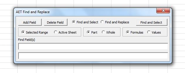
A multi-field Find and Select/Replace tool.

AET Find and Replace

Although a bit old, (like me), some of the code came from this.

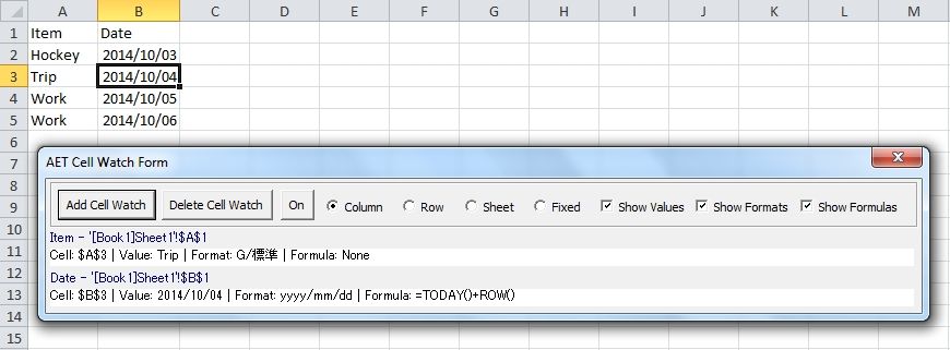
AET Cell Watch Form

Here’s the old post about it from back in 2009. (From my former blog, which I’ll also pimp!)

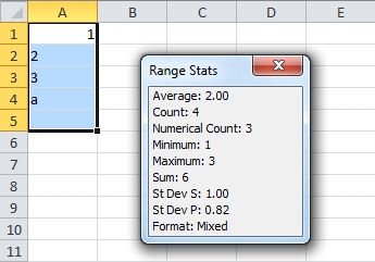
An alternative Status Bar that recognizes numbers even if the format is text. Woohoo!

AET Status Bar

And some games. (For the kids, but you can play too)
Grrr...
That’s enough pimpin’ for now. (I’m making new stuff as I write this) See you next time?

Data Comparison Tricks

Hey Dick, thanks for having me over. Wow, it’s even nicer in here than I imagined. Look at all those posts! Hey, is that an Office XP beer stein… where’d you get that? Gosh, do you really wear all these baseball caps?

Okay, well great to be here. I hope I don’t blow it. I’m going to talk about a fairly pedestrian topic, but one I deal with daily as a data analyst and report writer: comparing versions of output data.

At my work we have a report modification and publication process to verify that they’re outputting reasonable results. A lot of times this means comparing a report to its previous published version and confirming that the outputs are identical before moving on with the process.

I’ll show some tricks I use to do these comparisons. Please note these examples all assume the data you’re comparing is easily re-creatable, e.g., it comes from a data connection or was exported from another tool. In other words, don’t do these tests on the only copy of your output!

The Most Basic of Tricks – Comparing Sums

One quick trick you’ve probably used is to grab an entire column of output and check its SUM in the status bar. Aside from comparing row counts, this is about as simple as it gets.
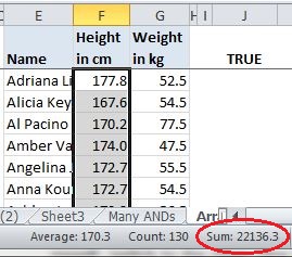
Status bar sum

I usually just look at the first three or so digits and the last three or so, mumble them to myself, switch to the other column and mumble those to myself. If my mumblings match, I call it good.

Mind you, I only do this as an informal check. Still, writing this got me to wondering how reliable it is, and about the likelihood of a false positive, a coincidental match. So I did a little test and filled two columns with RandBetween formulas then wrote a bit of VBA to recalculate them repeatedly and record the number of times their sums matched. With two columns of 1000 numbers, each filled with whole numbers between 1 and 1000, I averaged around three matches per 100,000 runs, or a .003% chance of a coincidental match. That’s a pretty small range of numbers though, equivalent to a span from one cent to ten dollars. So I upped it to whole numbers between one and a million, similar to one cent to 10,000 dollars. With a million calculations of 1000 rows there were no coincidental matching totals.

A More Thorough Trick – Compare All Cells

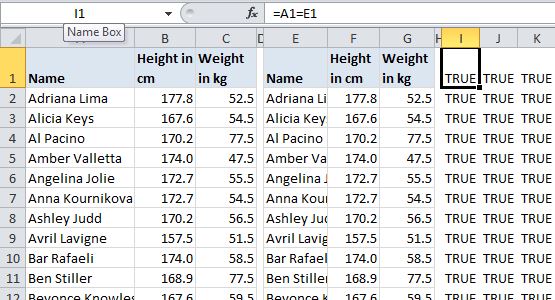
When I really want to make sure two sets of data with the same number of rows and columns match cell for cell, I do the obvious and … compare every cell. That could look something like this (but eventually won’t, so stick with me):
AND compare 1

The two sets of data (a modified version of the indispensable table from celeb-height-weight.psyphil.com) are on the left, with the comparison formulas for each cell on the right. In this case they all match and return TRUE:

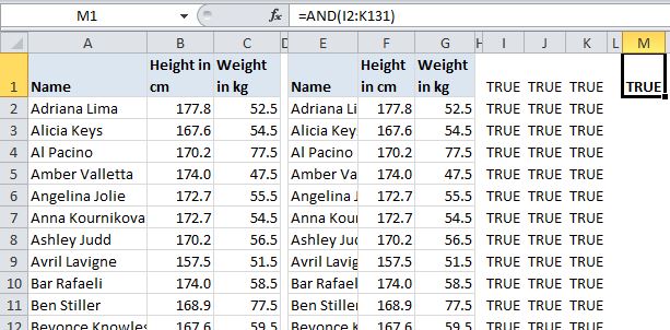
If you’ve got more than a few columns and rows, you probably don’t want to scan all the comparison cells for FALSEs. Instead, you can wrap up all these comparisons in a single AND, like this. It will return FALSE if any of the referenced cells are FALSE:
AND compare 2

Or just eliminate the middleperson altogether with a single AND in an array formula:
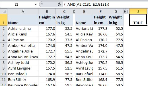
AND compare 3

What If They Don’t All Match?

If they don’t all match you can add conditional formatting to highlight the FALSEs…
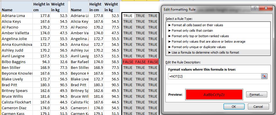
Conditional Formatting for FALSEs

… or just add it directly to the two tables. However, rather than conditional formatting I’d use a per-row AND array formula and filter to FALSE:
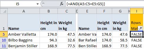
per-row ANDs

Same Data, Different Order

Sometimes my rows of data are the same, but they’re out of order. I try not to yell at them like Al Pacino. Instead I might test them with a COUNTIF(S) formula, like so, which just counts how many times the name in a the second table appears in the first table:

=COUNTIF($A$2:$A$131,E2)

To compare whole rows, you’re stuck (I think) with longer COUNTIFS formulas than I care to deal with. I’d rather concatenate the rows and compare the results with a COUNTIF. I don’t have many worksheet UDFs in my tools addin, but one exception is Rick Rothstein’s CONCAT function, which I found on Debra’s blog. It’s great because, unlike Excel’s Concatenate function, it allows you to specify a whole range, rather than listing each cell individually.

COUNTIFs can get slow though once you’ve got a few thousand rows of them. So, another approach is just to sort the outputs identically and then use an AND to compare them. Here’s a function I wrote to sort all the columns in a table:


Sub BlindlySortTable()
Dim lo As Excel.ListObject
Dim loCol As Excel.ListColumn

Set lo = ActiveCell.ListObject
With lo
.Sort.SortFields.Clear
For Each loCol In .ListColumns
.Sort.SortFields.Add _
Key:=loCol.DataBodyRange, SortOn:=xlSortOnValues, Order:=xlAscending, DataOption:=xlSortNormal
Next loCol
With .Sort
.Header = xlYes
.MatchCase = False
.Apply
End With
End With
End Sub

At this point I should mention that I almost always work with Tables (VBA ListObjects) when doing these comparisons. A lot of the time I’ve stuffed the SQL right into the Table’s data connection. If the data is imported from something like Crystal Reports, I’ll convert it to a table before working with it.

Using Pivot Tables For Comparing Data – Fun!

As I get farther along in a report’s development, odds are I might just want to compare a subset of the old version to the whole new version, or vice-versa. Using pivot tables is great for this. Say for instance my new report is only for people whose weight is under 48 kilograms. I’d like to compare the output of the new report to a filtered list from the older version and confirm that I’m returning the same weights for the people in the new subset. A pivot table makes this easy:
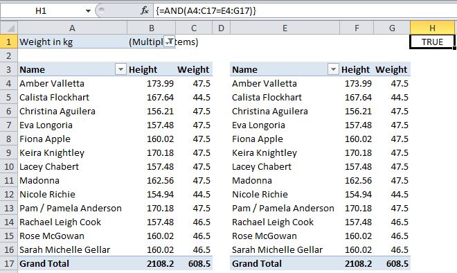
Pivot compare

The pivot on the left, based on the original data, has been filtered by weight and compared to the pivot on the right, based on the new, less-than-48 data. An AND formula confirms whether the data in the new one matches the original.

I was doing this the other day with multiple subsets, causing the pivots to resize. I thought “wouldn’t it be cool to have a function that returns a range equal to a pivot table’s data area?” The answer was “yes,” so I wrote one. It returns either the used range or the data area of a table or pivot table associated with the cell passed to it. Here’s the code:


Public Enum GetRangeType
UsedRange '0
'CurrentRegion - can't get to work in UDF in worksheet, just returns passed cell
PivotTable '1
ListObject '2
End Enum

Public Function GetRange(StartingPoint As Excel.Range, RangeType As GetRangeType) As Excel.Range
Dim GotRange As Excel.Range

With StartingPoint
Select Case RangeType
Case GetRangeType.UsedRange
Set GotRange = .Worksheet.UsedRange
Case GetRangeType.PivotTable
Set GotRange = .PivotTable.TableRange1
Case GetRangeType.ListObject
Set GotRange = .ListObject.Range
End Select
End With
Set GetRange = GotRange
End Function

The array-entered formula in H1 in the picture above becomes…

=GetRange(A3,1)= GetRange(E3,1)

… where 1 is a pivot table. You’ll note that the code itself uses the enum variable, which would be great if you could use the enums in a UDF. Also, you’ll see that I tried to have a cell’s CurrentRegion as an option but that doesn’t work. When returned to a UDF called from a worksheet, CurrentRegion just returns the cell the formula is in.

So Long

Okay then, see you later Dick. Thanks again for the invite. It means a lot to me.

No, no, don’t get up… I can show myself out and it looks like you’re working on something there. Wait a minute… no it couldn’t be… for a second there it looked like you were using a mouse… Must have been a trick of the light.

Cheers!

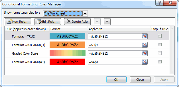
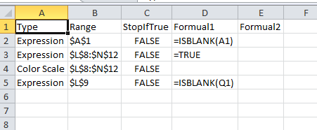
Listing Conditional Formatting Redux

Back in the day, I posted some code to list conditional formatting. It didn’t contemplate having multiple conditional formats for the same range. Because who would ever do that right? Of course that happens all the time and was very short-sighted of me. I aim to atone.

I used a Collection object because Collection objects can’t have two Keys that are the same. It’s a good way to get a unique list out of a list that contains duplicates. I used the range to which the FormatCondition applies as the key (and that was my downfall). My thought was this: I’m checking each cell individually and a FormatCondition that spans two cell would be counted twice. A FormatCondition that applied to L9:M9 would be counted for L9 and M9. By using the address as my unique key, it would only be counted once – the first time for L9 and it would error out and not be counted for M9.

Except you can have two FormatConditions that apply to L9:M9 and only the first would every be counted. I needed a way to identify what was a duplicate and what was a legitimate second FormatCondition. I cleverly devised (read stole from Bob Phillips) that I would add the count to the end of the address. But I got lucky in that it failed for my particular setup. The way my FormatConditions were created, they weren’t in the same order for all the cells. So even though an FC was the same for a later cell, it was the 3rd FC instead of the 2nd, and that made it seem unique.

I set out to find a better way to uniquely identify FCs, and here it is

It’s still no guarantee of uniqueness, but if you have two FCs with the same range, the same type, and the same formula, well, you gets what you deserves. Now I can use the ‘signature’ instead of the address.

And in case you forgot, here’s how I got the type.

Now this

gets you this

Converting Numbers to Words Part V

See Converting Numbers to Words Part IV

No need to bite this one off in small chunks. Just need to make sure the triplets processing works at the next level.

I’m just going to add a new If block for millions that looks a lot like the thousands If block. Of course I’ll be using exponents so I don’t have to type all those zeros.

All tests passed. The rest should be easy. I’m going to go a little sparse on the next tests.

I could create a new If block for each triplet, but I already know I’ll be refactoring, so what’s the point. I need to loop through however many triplets are there and process them.

Error: Overflow. I originally passed in a Double so I could do decimals, but never did the decimals. Anyway, it’s the integer division operator (\) that’s causing the problem. When you use a floating point number, like a Double, in an integer division expression, VBA casts it as a Long first. So anything more than 2.4 billion won’t work. Fortunately, MS has a fix.

All tests passed. And that’s it. I could add decimals, I suppose. Or even larger numbers.

The test-first methodology was pretty enjoyable, I have to say. This isn’t especially complicated code, but biting it off in small chunks made things flow nicely.

Converting Numbers to Words Part III

See Converting Numbers to Words Part II

My tests work from 0-99. The next test will test numbers between 100-199.

A haphazard selection of numbers including the edge cases.

And all tests pass. Back in the first post of this series I said that I hoped it would be obvious when I need to refactor. Well if this isn’t a frying pan to the face, I don’t know what is. Way too much repetition, for one. I need to introduce a “remainder” variable, so that once I process the hundred part, I can send the remainder to process the tens, and the remainder from that to the less than 19 part.

That looks much better, but it doesn’t pass the zero test. I don’t like special cases, but zero might just be one, so I’m going to force it. My conditional on whether to include a hyphen checks to see if the answer so far ends in “y”. That seems a little hokey, but it works. I could test for mod10 and set a Boolean variable in the If block above, but I’m not sure what I gain, so there it stays.

Refactoring in this way also makes the next bit of testing code painfully obvious. I’m hardcoding “one hundred”, but with vaSingles sitting right there, I don’t know why I can’t go above 199 pretty easily. So I’ll write that next test.

Instead of hardcoding “one hundred”, I’ll pull the property number from vaSingles. This also shows my brute force zero fix.

All tests pass. And the code doesn’t look too bad. Only infinity numbers left to test. Here’s what my main testing procedure looks like now, as if you couldn’t guess.

Converting Numbers To Words Part II

See Converting Numbers To Words Part I.

The next test will test 20-99. I think in real TDD, you’re supposed to write tests that test just one thing. But I’m not doing real TDD, so I’m testing in groups.

Again, I’m testing the edges and few in between. Now that I have two test procedures, I’ll need to create a procedure to run them both.

Now I can run TEST_All and make sure I don’t break any previous tests with the changes I make. Of course, TEST_Tens fails so it’s time to write some code to make it pass. I tried to write the simplest code possible, but it didn’t work out for me.

That fails because NumbersToWords(20) returns twenty-zero. So there’s a special case that needs to be handled.

That works. But I can see this special case handling becoming a problem. Maybe. We’ll see what happens when we test in the hundreds.

Converting Numbers To Words Part I

I overheard two people talking, one of whom was showing his intellectual prowess using that puzzle whose answer is always ‘four’. I don’t remember the specifics of the game, but you count the letters of an integer, do some basic math, and you always end up with ‘four’ because the word ‘four’ has that many letters in it. I get how it works, but I thought there’s surely another number with that property. Off to VBA to find out.

There’s not. But let me back up a bit. I searched the vast DDoE archives to find my Numbers-to-Words code. I’ve already written this code right? Apparently not. A broader search showed plenty of hits and, I’m sure, code, but I didn’t click any of the links. I’ve been hankering to write some test-first code and this seemed like a good candidate. I didn’t want to read anybody else’s code so it wouldn’t influence my test-first experience.

I’m going to document my test-first methodology in a series of posts. This is not test driven development (TDD), but borrows some of the principles from that. Basically, I write a test, watch it fail, then write enough code to make it pass. I refactor the code as necessary. If you are interested in TDD in Excel and VBA, search for xlUnit on Mike Woodhouse’s blog.

On to test 1! The idea is to write a function that returns a string that represents the English words of the argument. The procedure header should look like this:

First, write a test.

I know that once I hit 20 a pattern will start emerging, so I’m going to start by testing up to 19. Now I have to write enough code to make this pass. That’s seems pretty easy.

When I run that test, it passes. I put all the words for zero to 19 in an array, then read the array. What could be easier? For my tests, I choose the two edge cases (0 and 19) and a couple in the middle. It’s not very rigorous, but what the heck. One of the benefits of a test-first approach is that you’re biting off a bigger problem in smaller chunks. No single code revision is particularly difficult, but when put together can be complex. The refactoring part will be the interesting part. I assume it will be apparent when it’s time to refactor (as it is in examples I’ve seen) but I’ve never done it before, so we’ll see.

Next time, I’ll test some ‘tens’.

Avoiding Date Conversion When Pasting an HTML Table

From Get Data From a Website…, MD comments:

However, the info in the table I copy is formatted ## / ## whereby # represents a number.
So when it tries to paste 10 / 10 in the worksheet for example, it auto-changes to 10/okt in my sheet.

This is a common problem that’s hard to solve. There’s no setting I can find in Excel that tells it to stop converting things that look like dates into dates. Since I’m reading in the data and putting it in the clipboard, I can just message the data before I do it. That’s not so easy when you just want to copy and paste, but if you’re using code, you may find the technique useful.

In the above linked post, I automated Internet Explorer to login to a website. I don’t automate Internet Explorer any more, preferring XML instead. But it doesn’t matter which you use. It all ends up in an HTMLDocument, so it’s the same from there. Also, this example doesn’t log into a webpage. It uses Contextures’ Sample Data.

Sub GetTableNoDateConversion()

Dim xHttp As MSXML2.XMLHTTP
Dim hDoc As MSHTML.HTMLDocument
Dim hTable As MSHTML.HTMLTable
Dim hCell As MSHTML.HTMLTableCell
Dim doClip As MSForms.DataObject

'Get the webpage
Set xHttp = New MSXML2.XMLHTTP
xHttp.Open "GET", "http://www.contextures.com/xlSampleData01.html"
xHttp.send

'Wait for it to load
Do: DoEvents: Loop Until xHttp.readyState = 4

'Put it in a document
Set hDoc = New MSHTML.HTMLDocument
hDoc.body.innerHTML = xHttp.responseText

'Find the third table
Set hTable = hDoc.getElementsByTagName("table").Item(2)

'Fix anything that looks like a date
For Each hCell In hTable.Cells
If IsDate(hCell.innerText) Then
hCell.innerText = "'" & hCell.innerText
End If
Next hCell

'put it in the clipboard
Set doClip = New MSForms.DataObject
doClip.SetText "" & hTable.outerHTML & ""
doClip.PutInClipboard

'paste it to the sheet
Sheet1.Select
Sheet1.Range("A1").Select
Sheet1.PasteSpecial "Unicode Text"

'Make the leading apostrophes go away
Sheet1.Range("A1").CurrentRegion.Value = Sheet1.Range("A1").CurrentRegion.Value

End Sub

Once I get the table into an HTMLTable object, I loop through all the HTMLTableCells to see if any of them looks like a date. If so, I put an apostrophe in front of it. The apostrophe is the Excel way to say “No matter what I type next, assume it’s text”. Except when you’re pasting special as Unicode Text. In that case, it doesn’t hide the apostrophe like it should. So the last line of the code is the equivalent of pressing F2 and Enter all the say down the column and forcing Excel to reevaluate its decision to ignore that apostrophe.