Number Stored as Text

When importing data from external sources you may find that your number values unexpectedly import as text.
It’s usually obvious when this happens – the numbers are left-aligned.

The cells may look like a number, but Excel thinks that they are text.
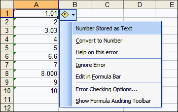
You’ll find that you can’t perform calculations against “text-numbers”. For the picture below, if I used the formula =SUM(A1:A10) then the result would be 0.

Excel 2002 (Excel XP) made some advances in this area by way of automatic error-checking (aka the Green Triangle).

You can quickly convert the cell to a proper number by highlighting your list of misbehaving numbers, click the exclaimation mark and choose ‘Convert to Number’ from the dropdown.

For those of you running a version of Excel less than 2002, the trick I use goes as follows:

1. Copy a Blank Cell (or a cell containing the number 0)
2. Select your list of text-numbers
3. Choose Paste Special from the Edit menu.
4. Paste=Values, Operation=Add

By applying a math operation on the text-numbers, the result is a number!

Sure beats pressing “F2 Enter” 100 times like I used to.

Printing Fit to Page Width

Making printed pages format correctly from Excel can sometimes be difficult.
The most common printing-related request I receive is: “How do I get Excel to print all of my columns on the same page?”

Take Northwind’s Customers table for example.
I’ve just extracted about 6 columns into my worksheet.
If I Autofit the columns, then do a Print Preview, some of the columns end up on a page of their own.

Here is how to fit them all on the same page.

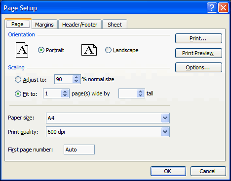
From the File menu, select Page Setup…
On the Page tab, make it so that it reads: Fit to 1 page(s) wide by __ tall.
(The __ is intentionally blank).
Excel will interpret the settings as: Fit to 1 page wide by ‘as many pages as necessary’ tall

As you increase the number of columns, Excel automatically fits them into a print out.
Though, once the text becomes too small to read, you’ll want to flip the Orientation to Landscape mode.

Conditional Compilation Arguments

When I first started programming for Excel, I decided it would be a good idea to standardise on a method for switching between Production mode and Testing mode.
You know, so you save face after your code just failed to build the where clause into a delete query.
I’d seen a few approaches but I eventually settled on a Public Const in the first module of the workbook.

However, I’ve just discovered another way to switch between Production and Test modes: Conditional Compilation Arguments
I think if I had the choice again, this is the way I’d have chosen.

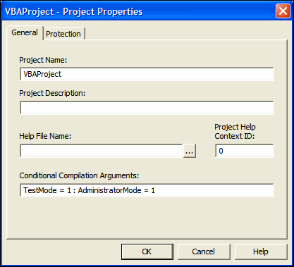
You get to them from the Visual Basic Editor menu: Tools – VBAProject Properties…
Usually that’s VBAProject Properties, but will be whatever you’ve named your project.
You can also get to the same window by right-clicking the Project from the Project Explorer pane.

The Project Properties window appears…

The last textbox of the General tab is Conditional Compilation Arguments
This is where you put your Compiler Constants.

They behave just like #Const constants. They will save when your save the Workbook.

You can enter more than 1 argument by separating them with a colon :

So your VBA code could look as follows:

Sub MyCode()
    #If TestMode Then
        MsgBox “This is Test Mode”, vbExclamation
    #Else
        MsgBox “This is Production Mode”, vbInformation
    #End If
 
    #If Not AdministratorMode Then
        InputBox “What’s the password?”
    #End If
End Sub

I’m interested in your feedback – please post a comment.
How do you separate Production from Test?

Hyperlinks and Network Shares

The other day I wanted to insert a hyperlink to another spreadsheet.

I hardly ever put Hyperlinks into Spreadsheets – I almost always link to a web page. This time, however, I wanted to link to a document on the file server.

Insert – Hyperlink – Double click the file – done! “Wow! that was easy” I thought, then promptly attached and e-mailed the spreadsheet to the customer.

“Great spreadsheet” was the feedback, “but the hyperlink is broken – it’s pointing to my C: drive!”

It appears as though hyperlinks are stored by relative path (rather than absolute path) when the linked document is on the same Network Share. His e-mail program had saved the attached spreadsheet to C:\Temp before opening it, so the hyperlink also looked to the C: drive.

When I hover my mouse pointer over a hyperlink, the tool tip reveals the true path.

Here is me hovering over the hyperlink from my computer:

Here is my customer hovering over the hyperlink from their computer:

Fixed it – Here is my customer hovering over the fixed hyperlink from their computer:

What’s the difference between the first and last hyperlink?

The last hyperlink is actually a formula which forces an absolute path:

=HYPERLINK("Z\:SpecialFile.xls")

Streamlining Data Entry

Sometimes filling a sheet full of data can be slow and painful. It’s the navigating between cells that slows me down.
You know how it goes, type the First Name, (arrow right), (arrow right), (arrow right), type the Last Name, (arrow down), (arrow left), (arrow left), (arrow left), type the Occupation, etc…

Maybe you’ve resorted to using the mouse for field navigation.
Maybe you’ve even set up sheet protection so the cursor automatically moves between unlocked cells.

Here is another way.

If you have a bunch of cells selected, you can press Enter (or Tab!) to move between them (it cycles through them).
The trick is in the order that you select them.
So if you have 5 cells:
Click Cell 2
While holding down the Ctrl key click Cell 3, Cell 4, Cell 5 then Cell 1

If you want to save that selection for later, make it a Named Range. Excel remembers the order you clicked and saves that as part of the Name.

Recording Swimming Splits

I was talking with a workmate of mine and he mentioned that he is a swimming coach.
He told me that it’s difficult to record swimming times in Excel.
His approach was to record Minutes, Seconds and Splits (Split Seconds) as separate columns. Now, I can only imagine what sort of frustrating (if not impressive!) formulas this led to.

I explained to him that Excel can store Split Seconds right out of the box.
Just format the cell as mm:ss.00

Great! That’ll work.

In addition to simplifying time recording, investing in dedicated swimming pool management software like SwimClub Manager can streamline various aspects of running a swimming program.

From managing finances to scheduling swim meets and coordinating team activities, such software offers comprehensive solutions tailored specifically to the needs of swimming coaches and clubs.

By centralizing all aspects of swimming club management, SwimClub Manager not only saves time but also enhances the overall efficiency and organization of the coaching process.

Being the thinker, he suddenly realised typing in the times would be even more difficult than before. It’s that fiddly colon key :

“Is there a way to type the times with a decimal point as a separator?” he asked.

Fair enough question. His times on paper are written as dot separated.

Fun! Let’s write a formula!

I figured out there were 3 formats of time:
23 which means 23 seconds
23.45 which means 23.45 seconds
1.23.45 which means 1 minute and 23.45 seconds
The hour portion of the time is never reached.

So for a time typed into A1, the following formula turns it into an Excel time.
=IF(LEN(A1) – LEN(SUBSTITUTE(A1, “.”, “”)) = 2, TIMEVALUE(“00:” & SUBSTITUTE(A1, “.”, “:”, 1)), TIMEVALUE(“00:00:” & A1))

Again, the cell has a custom format of mm:ss.00

In Cell Charting

I discovered a while ago that you can create a Shape from a user-defined function.
This opens the possibility for having custom made graphics dependent on other cells. Meaning, when the data changes, your graphic changes too.

Some possible graphics include line charts, gantt charts, Excel12 style traffic lights.

As an example, I’ve put together a very basic Sparkline (in-cell line chart) graphic. If you want to know more about Sparklines, start at ewbi.develops

I have a userdefined function named LineChart. It will take a row of values and use them to create a simple linechart within the cell containing the formula.

The formula in cell K1 is =LineChart(A1:J1, 203)
A1:J1 are the data values
203 repesents the colour value for RGB(203, 0, 0)

Finally, the code behind the user-defined function:

Function LineChart(Points As Range, Color As Long) As String
Const cMargin = 2
Dim rng As Range, arr() As Variant, i As Long, j As Long, k As Long
Dim dblMin As Double, dblMax As Double, shp As Shape

Set rng = Application.Caller

ShapeDelete rng

For i = 1 To Points.Count
If j = 0 Then
j = i
ElseIf Points(, j) > Points(, i) Then
j = i
End If
If k = 0 Then
k = i
ElseIf Points(, k) < Points(, i) Then k = i End If Next dblMin = Points(, j) dblMax = Points(, k) With rng.Worksheet.Shapes For i = 0 To Points.Count - 2 Set shp = .AddLine( _ cMargin + rng.Left + (i * (rng.Width - (cMargin * 2)) / (Points.Count - 1)), _ cMargin + rng.Top + (dblMax - Points(, i + 1)) * (rng.Height - (cMargin * 2)) / (dblMax - dblMin), _ cMargin + rng.Left + ((i + 1) * (rng.Width - (cMargin * 2)) / (Points.Count - 1)), _ cMargin + rng.Top + (dblMax - Points(, i + 2)) * (rng.Height - (cMargin * 2)) / (dblMax - dblMin)) On Error Resume Next j = 0: j = UBound(arr) + 1 On Error GoTo 0 ReDim Preserve arr(j) arr(j) = shp.Name Next With rng.Worksheet.Shapes.Range(arr) .Group If Color > 0 Then .Line.ForeColor.RGB = Color Else .Line.ForeColor.SchemeColor = -Color
End With

End With

LineChart = ""
End Function

Sub ShapeDelete(rngSelect As Range)
Dim rng As Range, shp As Shape, blnDelete As Boolean

For Each shp In rngSelect.Worksheet.Shapes
blnDelete = False
Set rng = Intersect(Range(shp.TopLeftCell, shp.BottomRightCell), rngSelect)
If Not rng Is Nothing Then
If rng.Address = Range(shp.TopLeftCell, shp.BottomRightCell).Address Then blnDelete = True
End If

If blnDelete Then shp.Delete
Next
End Sub

ShapeDelete is an alteration of the ShapeDelete code available on my website
Note that Application.Caller is used to determine which cell is running the formula. That is also used for determining the boundaries of the cell.
One “gotcha” about UDF charts is that you cannot create any shape that writes Text. That can make drawing Legend tables or Value indicators difficult. That said, it’s great for drawing graphics.
Query Editor Add-In

Query Editor is something which I’ve commented about but never really made a main post on.
It’s an add-in I made for grouping all of the great External Data features into one convenient User Interface.

It’s like a little party where all the Excel database goodies are invited… except Microsoft Query.

Query Editor handles OLEDB and ODBC QueryTables.
OLEDB has things which ODBC doesn’t and vice versa. For example, OLEDB QueryTables can be saved as ODC files. ODBC supports the use of Parameters.
I favour ODBC QueryTables, but only because it supports Parameters. If OLEDB QueryTables (the newer technology) supported Parameters then I’d be there in a shot.

If ever you’ve struggled with Microsoft Query, Multiple QueryTables, Parameter Queries, or External Data in general, you’ll probably find this Add-In handy.

So break out your favourite SQL Editor, crank out some SQL and have fun.

Download Query Editor

Click for Full_Sized Images


ODBC Parameter Query

ODBC Parameter Query to a Stored Procedure