Making a Wiki Table

Writing for Wikipedia is a bit like writing in your third language—you know there are words for it, but your guides are from your second language—Wiki pour Les Nuls or maybe Wiki para Maniquíes. It’s a different dialect of HTML. Having done it for several years, Wikipedia’s goal seems to be a reduction in keystrokes to be saved on its servers. For example, to italicize, rather than using the i- or em- tags, you use paired apostrophes (not double-quotes) to lead and close, saving at least three key strokes. To embolden, you use three apostrophes to lead and close, saving at least one stroke over the b- or strong- tags. And bold italics is thus five apostrophes leading, five apostrophes closing, saving at least four strokes. An unordered list’s members are just lines started with an asterisk, and an ordered list’s members are lines started with a pound sign. This economy follows into Wiki tables, where pipes (“|”) and curly braces (“{}”)are used for all the tags. There is a good summary of the table markup differences here. This little table:

1 2
3 4

 
In Wiki is this:

{|
| 1 || 2
|-
| 3 || 4
|}

as opposed to this:

1 2
3 4


If you have a table like this is in your spreadsheet:

Sports Teams    
  Boston New York
Baseball Boston Red Sox New York Yankees<br />New York Mets
Football New England Patriots New York Giants<br />New York Jets
Basketball Boston Celtics New York Knicks<br />New York Nets
Hockey Boston Bruins New York Rangers<br />New York Islanders

 
The MakeWikiTable() macro will make a table like this for Wikipedia:

Sports Teams
  Boston New York
Baseball Boston Red Sox New York Yankees
New York Mets
Football New England Patriots New York Giants
New York Jets
Basketball Boston Celtics New York Knicks
New York Nets
Hockey Boston Bruins New York Rangers
New York Islanders

And this table G33:H38

  G H I J K
32 Testing Sorting        
33 Coins Value      
34 Pennies 0.01<font color=white>[-]</font>   0.01 <font color=white>[-]</font>
35 Nickels 0.05<font color=white>[-]</font>   0.05 <font color=white>[-]</font>
36 Dimes 0.10<font color=white>[-]</font>   0.1 <font color=white>[-]</font>
37 Quarters 0.25<ref name=two>Two bits</ref>   0.25 <ref name=two>Two bits</ref>
38 Halves 0.50<ref name=four>Four bits</ref>   0.5 <ref name=four>Four bits</ref>

 
where H34: = Text(J34, "0.00") & K34 is aligned right and filled down, looks like this:

Testing Sorting
Coins Value
Pennies 0.01[-]
Nickels 0.05[-]
Dimes 0.10[-]
Quarters 0.25[1]
Halves 0.50[2]

Tapping into the class = “wikitable”, MakeWikiTable() can make any combination of sortable, collapsible, and collapsed tables. It invokes the class if the upper left table cell is not empty, and thus your (literally) first column is data vice row headers. There is a longstanding bug in the wikitable class that disables sorting if there is too much adornment given the table, no matter if the table is set as “sortable” or not. The combinations look like this in Wikipedia:

Only
Sorting
With Sorting
Collapsible
With Sorting
Collapsed
No Sorting
Collapsible
No Sorting
Collapsed
Coins Coins [hide] Coins [show] Coins [hide] Coins [show]

All these examples are available here. You’ll see the footnotes you created in Excel are at the bottom of the Wiki page. It looks different at Wiki Commons, but the code still works. Examples of a tables I made there with MakeWikiTable() are these. You’ll see it uses a sideways arrow instead of text for hide and show.

This is the MakeWikiTable code:

Public Sub MakeWikiTable()
Const DQ As String * 1 = """" 'double double double-quotes
Dim DataObj As New MSForms.DataObject
'Check VBE Tools/References Microsoft Forms 2.0 Object Library
Dim Rng As Range
Dim Cell As Range
Dim sReturn As String
Dim TextAlign As String
Dim CellContents As String
Dim UseRowHeaders As Boolean
Dim R As Long, C As Long
Dim IsSortable As Long, IsCollapsible As Long, IsCollapsed As Long
Dim Caption As String
Dim BgColor As String, FontColor As String

Set Rng = Selection
R = Rng.Rows.Count
C = Rng.Columns.Count

Caption = Rng.Cells(1, 1).Offset(-1, 0).Text 'Don't start the table in Row(1)
If Len(Rng.Cells(1.1)) = 0 Then
UseRowHeaders = True
IsSortable = vbNo
Else
IsSortable = MsgBox("Use Sortable Headers for your " & R & "-row by " & C & "-column table?", _
vbYesNoCancel + vbQuestion, "MRT's Wiki Table Maker")
If IsSortable = vbCancel Then Exit Sub
IsCollapsible = MsgBox("Do you want your table to collapse?", _
vbYesNoCancel + vbQuestion + vbDefaultButton1, "MRT's Wiki Table Maker")
If IsCollapsible = vbCancel Then Exit Sub
If IsCollapsible = vbYes Then
IsCollapsed = MsgBox("Do you want your table to load as collapsed?", _
vbYesNoCancel + vbQuestion + vbDefaultButton1, "MRT's Wiki Table Maker")
If IsCollapsed = vbCancel Then Exit Sub
End If
End If

If IsSortable = vbYes Or IsCollapsible = vbYes Then
sReturn = "{|class=" & DQ & "wikitable" & IIf(IsSortable = vbYes, " sortable", "") & _
IIf(IsCollapsible = vbYes, " collapsible", "") & _
IIf(IsCollapsed = vbYes, " collapsed", "") & DQ & _
" style=" & DQ & "margin: 1em auto 1em auto;" & DQ & vbNewLine
Else
sReturn = "{|border=" & DQ & "1" & DQ & " cellpadding=" & DQ & "5" & DQ & " cellspacing=" & DQ _
& "0" & DQ & " style=" & DQ & "margin: 1em auto 1em auto;" & DQ & vbNewLine
End If
sReturn = sReturn & "|+'''" & Caption & "'''" & vbNewLine
sReturn = sReturn & "|-" & vbNewLine

For Each Cell In Rng.Rows(1).Cells
CellContents = Cell.Text
If Len(CellContents) = 0 Then
CellContents = " "
Else
CellContents = Application.WorksheetFunction.Trim(CellContents)
End If
BgColor = HexColor(Cell.Interior.Color)
FontColor = HexColor(Cell.Font.Color)
sReturn = sReturn & "!scope=" & DQ & "col" & DQ & " style=" & DQ & "background-color:" & _
BgColor & "; color:" & FontColor & ";" & DQ & "| " & _
CellContents & vbNewLine
Next Cell

For R = 2 To Rng.Rows.Count
sReturn = sReturn & "|-" & vbNewLine
For C = 1 To Rng.Columns.Count

Set Cell = Rng.Cells(R, C)
CellContents = Cell.Text
If Len(CellContents) = 0 Then CellContents = " "

CellContents = MakeFracs(CellContents)
CellContents = Application.WorksheetFunction.Trim(CellContents)
CellContents = VBA.Replace(CellContents, "0 / 0", "zero / zero", 1, 1, vbTextCompare)

If C = 1 And UseRowHeaders Then
BgColor = HexColor(Cell.Interior.Color)
FontColor = HexColor(Cell.Font.Color)
sReturn = sReturn & "!scope=" & DQ & "row" & DQ & " style=" & DQ & "background-color:" & _
BgColor & "; color:" & FontColor & ";" & DQ & "| " & _
CellContents & vbNewLine
Else
Select Case Cell.HorizontalAlignment
Case xlGeneral
TextAlign = "left"
If IsNumeric(Cell.Value) Then TextAlign = "right"
If IsError(Cell.Value) Then TextAlign = "center"
Case xlLeft
TextAlign = "left"
Case xlCenter
TextAlign = "center"
Case xlRight
TextAlign = "right"
Case xlJustify
TextAlign = "center"
End Select

sReturn = sReturn & "|align=" & TextAlign & "| "
With Cell.Font
If .Italic Then sReturn = sReturn & "''"
If .Bold Then sReturn = sReturn & "'''"
End With

sReturn = sReturn & CellContents

With Cell.Font
If .Bold Then sReturn = sReturn & "'''"
If .Italic Then sReturn = sReturn & "''"
End With

sReturn = sReturn & vbNewLine
End If
Next C
Next R

sReturn = sReturn & IIf(IsSortable = vbYes, "|-class=sortbottom" & vbNewLine, "")
sReturn = sReturn & "|}" & vbNewLine

DataObj.SetText sReturn
DataObj.PutInClipboard

End Sub

Function HexColor(Color As Long) As String
Dim Red As String, Green As String, Blue As String
Red = VBA.Hex(Color And 255)
Green = VBA.Hex(Color \ 256 And 255)
Blue = VBA.Hex(Color \ 256 ^ 2 And 255)
If Len(Red) = 1 Then Red = "0" & Red
If Len(Green) = 1 Then Green = "0" & Green
If Len(Blue) = 1 Then Blue = "0" & Blue
HexColor = "#" & Red & Green & Blue
End Function

Note that the Caption is at Offset(1,0) from the your selected table. Wikipedia’s examples all use muted grays for the headers. The first two of the following are the provided colors, the third, aka “silver” is what I used above.

#EFEFEF #CFCFCF #C0C0C0

The macro should be invoked from a form instead of daisy-chained message boxes. I got lazy. The MakeFracs() function is here. If you want to put something in the upper-left cell, and still get row headers, put it in after you paste your table into Wikipedia.

… mrt
©¿©¬
Turning an Excel table into CSS

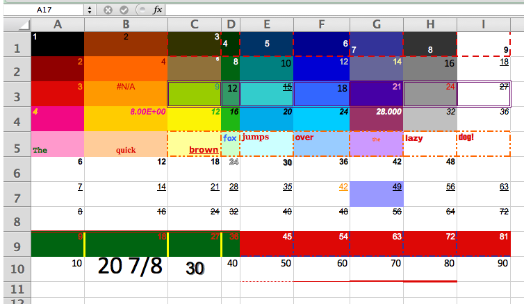
This is my very ugly, very formatted, table to test my translation skills, first into HTML and now into CSS. Every cell has at least two formats that have a counterpart in CSS, and the table runs through all options at some point.

Ugly Table

 
Row(5) has nine different fonts, at assorted alignments, from left to right:

  • Courier New
  • Time New Roman
  • Verdana
  • Comic Sans MS
  • Georgia
  • Tahoma
  • Trebuchet MS
  • Arial Black
  • Impact

I think Microsoft Office puts those fonts on every machine. A1:H5 are the colors of the old/original color pallate. This is my CSS rendering of the double-ugly table.

  A B C D E F G H I
1 1 2 3 4 5 6 7 8 9
2 2 4 6 8 10 12 14 16 18
3 3 #N/A 9 12 15 18 21 24 27
4 4 8.00E+00 12 16 20 24 28.000 32 36
5 The quick brown fox jumps over the lazy dog!
6 6 12 18 24 30 36 42 48  
7 7 14 21 28 35 42 49 56 63
8 8 16 24 32 40 48 56 64 72
9 9 18 27 36 45 54 63 72 81
10 10 20 ⅞ 30 40 50 60 70 80 90
11                  

 
Tricks were required to capture conditional formatting, which is not contained in a cell’s styling. From here, Chip Pearson showed me the way. The mental picture I formed was of conditional formatting floating in a horizontal plane above the spreadsheet, hiding the “regular” formatting below it. Reverse engineering the way cell formats interact with conditional formats was not fun, but the result should be near to what you see in your spreadsheet. Several cells in Row(7) are conditionally formatted. Browsers can screw this up. The bottom border of E10 is a dotted red line. It’s set as xlHairline in the spreadsheet. The HTML properly specifies it as a dotted red line, and outside of WordPress, that’s what I see. Just not here. Similarly, I’ve specified the column widths and their max-widths. WordPress doesn’t seem to care, and spreads the table 100%. My impression is that inline styles win, but not always on WordPress, I guess.

The graphic is about 70KB and the table about 57KB. While the graphic will be always be around 70KB, the table will shrink as formatting is lessened. For the 120 cells above, which includes the heading cells, that’s about 486 bytes per cell. To speed the concatenation up, I implemented (the late) Nate Oliver’s buffer concept, with a buffer for 106 characters, or room for over 2,000 excessively formatted cells.

The MakeCSSTable() procedure looks at the selected cells from left to right, top to bottom, and aligns each cell’s attributes with CSS. Except for the optional case of not capturing the headers, only the bottom and right borders are captured (the left and top being captured from a previous cell). When no-headers are chosen, all four borders are captured for the top row and left column. Someone please speakup if it’s documented what the layout or z-order for Excel’s cells is, and how their borders overlay. I think I got close to right, but since the browsers may do it differently, I’m not sure. If you change your gridline settings, MakeCSSTable() follows along.

My initial approach gave a CSS style for each attribute on each edge. As I got smarter, I grouped the the attributes into shortcuts. Not every Excel attribute has a CSS counterpart. For instance, diagonal borders do not exist in CSS, CSS only offers one kind of underlining, CSS3 adds an outline font but browsers don’t handle it yet (see Cell(D6)—it’s in the macro though for when they do), and Excel has more dashed/dotted line styles than CSS. Predominately dashed styles align to a “dashed” CSS style, with a similar arrangement for dotted lines. Things I stumbled upon in doing this: Column widths are a pixel measurement (based on the Normal-style font size) and row heights are a point measurement. For small Excel font sizes (<11) I specified a CSS use of a value of “small” in one line’s code. Since this is outside what Excel calculated, it can throw the column widths off. You can see the difference in the G5 cells.

This little table:

  A B
17 1 2000
18 3000 4
19 5 38 ⅞

 
Looks like this underneath:

  A B
17 1 2000
18 3000 4
19 5 38 ⅞


The CSS_Tablemaker module is 700+ lines of code, including the whitespace, so it’s available here as a spreadsheet file. It comes complete with the MakeCSSTable(), AddToBuffer(), MakeFracs(), and HexColor() routines, and as much of Chip’s code as I used. The absolutely stunning tables above are included, no charge. The header details are module constants you can adjust. The output is dumped to the clipboard to paste where you want.

 
… mrt
©¿©¬

Using HTML5 Fractions in Exported Excel Tables

HTML5 provides for fractional representation of halves, thirds, fourths, fifths, sixths, no sevenths, and eighths. Excel has a fractional number format. This post is about bringing these concepts together for exporting an Excel table into Wiki or HTML designs. The basic representations are:

Name Hex Dec Result
&frac12; U+000BD 189 ½
&frac13; U+02153 8531
&frac14; U+000BC 188 ¼
&frac15; U+02155 8533
&frac16; U+02159 8537
&frac18; U+0215B 8539
&frac23; U+02154 8532
&frac25; U+02156 8534
&frac34; U+000BE 190 ¾
&frac35; U+02157 8535
&frac38; U+0215C 8540
&frac45; U+02158 8536
&frac56; U+0215A 8538
&frac58; U+0215D 8541
&frac78; U+0215E 8542

 
The format for the name is &fracnd; where n is the numerator and d is the denominator. Thus &frac12; is a half, and &frac78; is seven-eighths. The HTML code representations for these are:

Result Named
Code
Hex
Code
Dec
Code
½ &frac12; &#X00BD; &#189;
&frac13; &#X2153; &#8531;
¼ &frac14; &#X00BC; &#188;
&frac15; &#X2155; &#8533;
&frac16; &#X2159; &#8537;
&frac18; &#X215B; &#8539;
&frac23; &#X2154; &#8532;
&frac25; &#X2156; &#8534;
¾ &frac34; &#X00BE; &#190;
&frac35; &#X2157; &#8535;
&frac38; &#X215C; &#8540;
&frac45; &#X2158; &#8536;
&frac56; &#X215A; &#8538;
&frac58; &#X215D; &#8541;
&frac78; &#X215E; &#8542;

 
In theory (more on “in practice” later) every representation in a row is equivalent. This is our test table to export to Wiki or HTML format:

D E F G H I J K L
1 1/1 1/2 1/3 1/4 1/5 1/6 1/7 1/8 1/80
2 2/1 2/2 2/3 2/4 2/5 2/6 2/7 2/8 2/8.
3 3/1 3/2 3/3 3/4 3/5 3/6 3/7 3/8 3/8A
4 4/1 4/2 4/3 4/4 4/5 4/6 4/7 4/8 6 4/8
5 5/1 5/2 5/3 5/4 5/5 5/6 5/7 5/8 7 5/8
6 6/1 6/2 6/3 6/4 6/5 6/6 6/7 6/8 8 6/8
7 7/1 7/2 7/3 7/4 7/5 7/6 7/7 7/8 9 7/8
8 8/1 8/2 8/3 8/4 8/5 8/6 8/7 8/8 10 8/8

 
Cell D1: =CHAR(32)&ROW()&”/”&COLUMN()-3, then fill down and right. The right hand column has a few test cases. I used that formulaic construction to keep Excel from doing the divisions. The Excel fractional format is “# ?/?” for single digit denominators. The intermediary space is important. It indicates that a fraction may follow, just as a forward slash indicates a fraction may be present. And a format of /?? is a fraction not translatable into HTML5. Turning these patterns into VBA, this is my MakeFracs() function. It checks that there is a slash, then that there is not a slash–digit–digit pattern, and finally that there is a “space–digits 1 through 7–slash–digits 2, 3, 4, 5, 6, 8” pattern to screen out sevenths and ninths. If all of those pass, it substitutes in the &fracnd; formulation for the fraction.

Function MakeFracs(Arg As String) As String
Dim sIN As String
Dim sOUT As String
Dim i As Long, j As Long
Dim n As Long, d As Long
Dim Fracs(1 To 15, 1 To 3) As String

Fracs(1, 1) = "½": Fracs(1, 2) = "½": Fracs(1, 3) = "½"
Fracs(2, 1) = "⅓": Fracs(2, 2) = "⅓": Fracs(2, 3) = "⅓"
Fracs(3, 1) = "¼": Fracs(3, 2) = "¼": Fracs(3, 3) = "¼"
Fracs(4, 1) = "⅕": Fracs(4, 2) = "⅕": Fracs(4, 3) = "⅕"
Fracs(5, 1) = "⅙": Fracs(5, 2) = "⅙": Fracs(5, 3) = "⅙"
Fracs(6, 1) = "⅛": Fracs(6, 2) = "⅛": Fracs(6, 3) = "⅛"
Fracs(7, 1) = "⅔": Fracs(7, 2) = "⅔": Fracs(7, 3) = "⅔"
Fracs(8, 1) = "⅖": Fracs(8, 2) = "⅖": Fracs(8, 3) = "⅖"
Fracs(9, 1) = "¾": Fracs(9, 2) = "¾": Fracs(9, 3) = "¾"
Fracs(10, 1) = "⅗": Fracs(10, 2) = "⅗": Fracs(10, 3) = "⅗"
Fracs(11, 1) = "⅜": Fracs(11, 2) = "⅜": Fracs(11, 3) = "⅜"
Fracs(12, 1) = "⅘": Fracs(12, 2) = "⅘": Fracs(12, 3) = "⅘"
Fracs(13, 1) = "⅚": Fracs(13, 2) = "⅚": Fracs(13, 3) = "⅚"
Fracs(14, 1) = "⅝": Fracs(14, 2) = "⅝": Fracs(14, 3) = "⅝"
Fracs(15, 1) = "⅞": Fracs(15, 2) = "⅞": Fracs(15, 3) = "⅞"

i = VBA.InStr(1, Arg, "/", vbTextCompare)
If i = 0 Then 'there's no fraction
MakeFracs = Arg
ElseIf Mid$(Arg, i, 3) Like "/##" Then 'not HTML5
MakeFracs = Arg
ElseIf Mid$(Arg, i - 2, 4) Like " [1-7]/[234568]" Then
sOUT = Mid$(Arg, i - 1, 3)
n = VBA.Val(Left$(sOUT, 1)) 'numerator
d = VBA.Val(Right$(sOUT, 1)) 'denominator
If n < d Then If d Mod n = 0 Then d = d / n n = 1 ElseIf d Mod 2 = 0 And n Mod 2 = 0 Then d = d / 2 n = n / 2 End If sIN = "&frac" & n & d & ";" For j = 1 To 15 If Fracs(j, 1) = sIN Then sIN = Fracs(j, 2) '<-or Fracs(j, 3) for HEX Exit For End If Next j MakeFracs = VBA.Replace(Arg, sOUT, sIN) Else MakeFracs = Arg End If Else MakeFracs = Arg End If End Function


At least that's all I wanted it to do. In practice, Wikipedia and WordPress seem to be not fully onboard with HTML5 and do not handle all fifteen &fracnd; formats (I confirmed Firefox does). That added "j-loop" in the middle translates the &fracnd;'s into Dec code. This works fine, though it's a step back from HTML5. Option is given to use Hex if desired. Your Excel table then looks like this:

N O P Q R S T U V
1 1/1 &#189; &#8531; &#188; &#8533; &#8537; 1/7 &#8539; 1/80
2 2/1 2/2 &#8532; &#189; &#8534; &#8531; 2/7 &#188; &#188;.
3 3/1 3/2 3/3 &#190; &#8535; &#189; 3/7 &#8540; &#8540;A
4 4/1 4/2 4/3 4/4 &#8536; &#8532; 4/7 &#189; 6 &#189;
5 5/1 5/2 5/3 5/4 5/5 &#8538; 5/7 &#8541; 7 &#8541;
6 6/1 6/2 6/3 6/4 6/5 6/6 6/7 &#190; 8 &#190;
7 7/1 7/2 7/3 7/4 7/5 7/6 7/7 &#8542; 9 &#8542;
8 8/1 8/2 8/3 8/4 8/5 8/6 8/7 8/8 10 8/8

 
Where N1: =MakeFracs(D1) filled down and right. Arranged that way you can see the HTML5 design thoughts. The very ugly website would look like this:

1/1 ½ ¼ 1/7 1/80
2/1 2/2 ½ 2/7 ¼ ¼.
3/1 3/2 3/3 ¾ ½ 3/7 ⅜A
4/1 4/2 4/3 4/4 4/7 ½ 6 ½
5/1 5/2 5/3 5/4 5/5 5/7 7 ⅝
6/1 6/2 6/3 6/4 6/5 6/6 6/7 ¾ 8 ¾
7/1 7/2 7/3 7/4 7/5 7/6 7/7 9 ⅞
8/1 8/2 8/3 8/4 8/5 8/6 8/7 8/8 10 8/8

 
Frankly, I'm not sure that this is an improvement. You'll come across Wikipedia editors, however, who are convinced of it. I thought about adding a trailing space, as in MakeFracs = VBA.Replace(Arg, sOUT, sIN & Chr(32)), but for every time I wanted to, I thought of an example where I didn't, and the logic got very convoluted. Better I decided to put the space in the table where wanted and not in the function. My HTML tablemaker is here, but it's being overcome by the hard steady march of technology. Wiki and CSS tablemakers are coming up. I used MakeFracs() in the above. No fractions were harmed in the making of this post.

…mrt
©¿©¬

A ‘Price is Right’ Algorithm

You’ve probably watched The Price is Right TV game show. On it they run the Clock Game.

The game is played for two prizes. The actual price of the first prize is shown to the studio and home audiences. After the contestant gives their first bid, a 30 second clock is started and the host tells the contestant whether the actual price is higher or lower than the bid. The contestant continues to bid, responding to the host’s clues, until either the contestant wins by correctly guessing the price of the prize or the time expires. If time remains after the first prize is won, the process is repeated for the second prize.…With few exceptions, only prizes valued below $1,000 have traditionally been offered in the Clock Game.

The algorithm to use is simple:

  • Pick a ceiling ($1000) and a floor ($0)
  • Bid the average ($500)
  • If the bid is too low, the bid becomes the floor
  • If the bid is too high, the bid becomes the ceiling
  • Repeat

Being computer types, we’ll put the ceiling at $1024. For a $407-priced prize, your guesses would look like this:

  C D E F
1   407 <-- Price  
2 Floor BID   Ceiling
3 0 512 Too High 1024
4 0 256 Too Low 512
5 256 384 Too Low 512
6 384 448 Too High 512
7 384 416 Too High 448
8 384 400 Too Low 416
9 400 408 Too High 416
10 400 404 Too Low 408
11 404 406 Too Low 408
12 406 407 Stop 408

 
Ten guesses, and you’ve won a washing machine. Here are the formulas that make this work.

  • D1: = 407 (the unknown price)
  • C3: = 0 (the initial floor)
  • F3: = 1024 (the initial ceiling)
  • D3: = (C3+F3)/2 (512—the initial bid)
  • E3: = IF(D3=$D$1,”Stop”,IF(D3>$D$1,”Too High”,”Too Low”)) (the host’s clues)
  • C4: = IF(E3=”Stop”,””,IF(E3=”Too Low”,D3,C3))
  • D4: = IF(E3=”Stop”,””,(C4+F4)/2)
  • E4: = IF(D4=$D$1,”Stop”,IF(D4>$D$1,”Too High”,”Too Low”))
  • F4: = IF(E3=”Stop”,””,IF(E3=”Too High”,D3,F3))

Watch out for “curly quotes” if you copy and paste in. Filldown C4:F13. So what’s the point? We knew the “unknown price” going in. Here’s a recent prospective employee question the BBC got from Qualcomm:

Given 20 ‘destructible’ light bulbs (which break at a certain height), and a building with 100 floors, how do you determine the height the light bulbs break?

You watch The Price is Right or you read DDoE, and you think “Clock Game!” In 20 bulbs, if they break from a 407.407 foot drop, and a floor = 10 feet:

    407.407 <-- Break  
  Floor BID   Ceiling
1 0 512 Too High 1024
2 0 256 Too Low 512
3 256 384 Too Low 512
4 384 448 Too High 512
5 384 416 Too High 448
6 384 400 Too Low 416
7 400 408 Too High 416
8 400 404 Too Low 408
9 404 406 Too Low 408
10 406 407 Too Low 408
11 407 407.5 Too High 408
12 407 407.25 Too Low 407.5
13 407.25 407.375 Too Low 407.5
14 407.375 407.4375 Too High 407.5
15 407.375 407.4063 Too Low 407.4375
16 407.4063 407.4219 Too High 407.4375
17 407.4063 407.4141 Too High 407.4219
18 407.4063 407.4102 Too High 407.4141
19 407.4063 407.4082 Too High 407.4102
20 407.4063 407.4072 Too High 407.4082

 
You’re 2-ten-thousandths of a foot off. You get the job, a great way to start the new year.

 
…mrt
©¿©¬

Working with the MAXIF() and LARGEIF() functions

Oh, Wait! Excel doesn’t have those functions. We’ll have to roll our own. We’re going to use the Double Unary tip found here. In Excel, 1*TRUE = 1, 0+TRUE = 1, TRUE^1 = 1, and minus-minus TRUE (–TRUE, the double unary) = 1. It’s two sign changes, and thought to be the best way to turn an array of TRUE/FALSE into ones/zeros. Multiplying an array of parameters by an array of ones and zeros leaves only the TRUE parameters non-zero.

Back to our list of the 122 major teams in professional sports, the Boss has decided that sorting by name length, then alphabetically, isn’t going to do. He wants it by name length by stadium size. So, thanks to Wikipedia, your data looks like this, Column(F) is arena size:

  D E F
1 Anaheim Ducks 13 17,174
2 Arizona Cardinals 17 63,400
3 Arizona Diamondbacks 20 48,633
4 Atlanta Braves 14 50,097
5 Atlanta Falcons 15 71,228
6 Atlanta Hawks 13 18,729
7 Baltimore Orioles 17 45,363
8 Baltimore Ravens 16 71,008
9 Boston Bruins 13 17,565
10 Boston Celtics 14 18,624

Using fzz’s comment about the ROW() function, we’ll sort the length by G1=LARGE($E$1:$E$122,ROWS($G$1:$G1)) filled down. The table looks much like before:

  D E F G
1 Anaheim Ducks 13 17,174 29
2 Arizona Cardinals 17 63,400 22
3 Arizona Diamondbacks 20 48,633 22
4 Atlanta Braves 14 50,097 22
5 Atlanta Falcons 15 71,228 21
6 Atlanta Hawks 13 18,729 21
7 Baltimore Orioles 17 45,363 21
8 Baltimore Ravens 16 71,008 20
9 Boston Bruins 13 17,565 20
10 Boston Celtics 14 18,624 20

We know there are only three teams of name length 22. A formula – -($E$1:$E$122=22), using the double unary operation, gives us an array of 119 zeros, and just 3 ones that line up on 22. If we multiply that array by the array of arena capacities (F1:F122) we have 119 multiplications by zero, and three multiplications by 1. A MAX() function or an equivalent LARGE(,1) function on that array product returns the capacity of largest stadium hosting a team name 22 letters long. Those equations formulas, array entered, would look like this:

  • {=LARGE(- -($E$1:$E$122=22)*$F$1:$F$122,1)}
  • {=MAX(- -($E$1:$E$122=22)*$F$1:$F$122)}

We want to modify those for different teams. Changing the =22 to =$G1 is a start, and we’ve gone about as far as we can with our ‘MAXIF().’ It’s going to return the same thing three times. A scheme using COUNTIF() starting from the top and working down will improve the ‘LARGEIF()’. Using mixed references, $G$1:$G1 will grow as we fill down. COUNTIF($G$1:$G2,$G2) will only count one 22, COUNTIF($G$1:$G3,$G3) will count two 22s, and COUNTIF($G$1:$G4,$G4) will count 3, and that’s all there are. This array-entered equationformula then, filled down, is ‘LARGEIF()’:

  • {=LARGE(- -($E$1:$E$122=$G1)*$F$1:$F$122,COUNTIF($G$1:$G1,$G1))}

In I1 filldown =MATCH(H1,$F$1:$F$122,0) and in J1 filldown =INDEX(D:D,I1). Your table should look like this:

  D E F G H I J K
1 Anaheim Ducks 13 17,174 29 45,389 52 Los Angeles Angels of Anaheim  
2 Arizona Cardinals 17 63,400 22 19,980 95 Portland Trail Blazers  
3 Arizona Diamondbacks 20 48,633 22 19,356 63 Minnesota Timberwolves  
4 Atlanta Braves 14 50,097 22 18,144 30 Columbus Blue Jackets  
5 Atlanta Falcons 15 71,228 21 43,651 89 Philadelphia Phillies  
6 Atlanta Hawks 13 18,729 21 19,596 42 Golden State Warriors  
7 Baltimore Orioles 17 45,363 21 18,203 83 Oklahoma City Thunder  
8 Baltimore Ravens 16 71,008 20 68,756 69 New England Patriots  
9 Boston Bruins 13 17,565 20 67,164 49 Jacksonville Jaguars  
10 Boston Celtics 14 18,624 20 65,857 108 Tampa Bay Buccaneers  

Column(I) shows the indices reordered by size of the arena.

There are some problems with this approach. It only works with positive numbers, such as our capacities. Negative numbers will be less than a FALSE, and a zero will be returned in their place. And if ever capacities are equal, it will always return only the first (same old problem). Nicely here, hockey and basketball held in the same arena draw to different capacity. The file is available at http://wl.filegenie.com/~JMOprof/LargeIF.xls

…mrt
©¿©¬

The Twelve Days of Excel

When you carol along with The Twelve Days of Christmas do you think of spreadsheets? I do, and that certainly says all you need to know about my musical ability. The folks at PNC Wealth Management do also. Annually they issue their Christmas Price Index, with the 2011 version here. Spreading the data out, The Twelve Days of Christmas looks like this:

A B C D E F G H I J K L M N O P
1   1st
Day
2nd
Day
3rd
Day
4th
Day
5th
Day
6th
Day
7th
Day
8th
Day
9th
Day
10th
Day
11th
Day
12th
Day
Total
Quantity
Unit Cost Bundled Cost
2 Drummers Drumming                       12 12 $ 219.16 $ 2,629.90
3 Pipers Piping                     11 11 22 $ 220.69 $ 2,427.60
4 Lords-a-leaping                   10 10 10 30 $ 476.67 $ 4,766.70
5 Ladies Dancing                 9 9 9 9 36 $ 699.34 $ 6,294.03
6 Maids-a-milking               8 8 8 8 8 40 $ 7.25 $ 58.00
7 Swans-a-swimming             7 7 7 7 7 7 42 $ 900.00 $ 6,300.00
8 Geese-a-laying           6 6 6 6 6 6 6 42 $ 27.00 $ 162.00
9 Golden Rings         5 5 5 5 5 5 5 5 40 $ 129.00 $ 645.00
10 Calling Birds       4 4 4 4 4 4 4 4 4 36 $ 129.99 $ 519.96
11 French Hens     3 3 3 3 3 3 3 3 3 3 30 $ 50.00 $ 150.00
12 Turtle Doves   2 2 2 2 2 2 2 2 2 2 2 22 $ 62.50 $ 125.00
13 Partridge 1 1 1 1 1 1 1 1 1 1 1 1 12 $ 15.00 $ 15.00
14 Pear Tree 1 1 1 1 1 1 1 1 1 1 1 1 12 $ 169.99 $ 169.99

PNC provides the Bundled Cost. We have to work backwards to find the Unit Cost. In other words, eight total maids-a-milking cost $58. The data sources are at the Wiki link. The poor dairy lasses are working minimum wage.

For DDoE, PNC’s table is a good way to review the concept of named ranges. Define Christmas as =Sheet1!$B$2:$M$14, _12th_Day as =Sheet1!$M$2:$M$14, Bundled_Cost as =Sheet1!$P$2:$P$14, Maids as =Sheet1!$B$6:$P$6, Quantity as =Sheet1!$N$2:$N$14, and Unit_Cost as =Sheet1!$O$2:$O$14.

The total number of gifts can be =SUM(Christmas) or =SUM(Quantity), being 376 (more on this later). The cost of the 12th Day of Christmas can be =SUM(Bundled_Cost) or = SUMPRODUCT(_12th_Day,Unit_Cost), being $24,263.18. The total expenditure of your True Love is =SUMPRODUCT(Quantity,Unit_Cost), or $101,119.84. A very generous person, your True Love.

We can use the Intersection Operator, a space, as =Maids Quantity, to find that we need 40 work hours from them. The value of named ranges is in the legibility it brings to your spreadsheet. You can expand this until you cover all days and all gifts. The work is in the defining of the names, the benefit is in the presentation.

PNC says the total gifts number 364. Surely a partridge and a pear tree count as two gifts in your household, no? Happy Holidays!

…mrt
©¿©¬

Finding the 2nd, 3rd, 4th … MATCH()

Excel’s MATCH() function will return the relative location of the first occurrence that satisfies the match criterion (the lookup_value) within the specified array (the lookup_array).  Most often, this is what you want.  For instance, if you have duplicate entries, returning the first match is no different than returning the last match.  However, if you have unique entries with the duplicated criterion, how do you return all the unique values?

For example, you have a list of the 122 major professional sports teams (32 NFL, and 30 MLB, NBA, and NHL) sorted alphabetically in Column D. Whichever sports team you may like, you have the access to bet on them thanks to sites such as 벳엔드 후기.  In Column E, you have code that returns the length of the team name, i.e. =LEN(D1).  Your data might look like this:

D E
1 Anaheim Ducks 13
2 Arizona Cardinals 17
3 Arizona Diamondbacks 20
4 Atlanta Braves 14
5 Atlanta Falcons 15
6 Atlanta Hawks 13
7 Baltimore Orioles 17
8 Baltimore Ravens 16
9 Boston Bruins 13
10 Boston Celtics 14

For no good reason we want to create a descending sort on name length. You can do it from the Sort selection, but we also want to keep the alpha-sort. In F1 you put =LARGE($E$1:$E$122,ROW()) and fill down. The ROW() function will cause the return of the first largest, then the second largest etc. Then you want to know how far down Column E those descending numbers fall, so that you can Index the name list that amount. In G1 put the code =MATCH(F1,$E$1:$E$122,0) and fill down. You’ll see from the data that the longest name is 29 letters, and it’s in ROW(52).

D E F G
1 Anaheim Ducks 13 29 52
2 Arizona Cardinals 17 22 30
3 Arizona Diamondbacks 20 22 30
4 Atlanta Braves 14 22 30
5 Atlanta Falcons 15 21 42
6 Atlanta Hawks 13 21 42
7 Baltimore Orioles 17 21 42
8 Baltimore Ravens 16 20 3
9 Boston Bruins 13 20 3
10 Boston Celtics 14 20 3

You can begin to see the problem: There are three teams with a 22-letter name, three with a 21-letter name, and at least 3 (in fact 13) with a 20-letter name. If in H1 we put =INDEX(D:D,G1) and filldown, we get:

D E F G H
1 Anaheim Ducks 13 29 52 Los Angeles Angels of Anaheim
2 Arizona Cardinals 17 22 30 Columbus Blue Jackets
3 Arizona Diamondbacks 20 22 30 Columbus Blue Jackets
4 Atlanta Braves 14 22 30 Columbus Blue Jackets
5 Atlanta Falcons 15 21 42 Golden State Warriors
6 Atlanta Hawks 13 21 42 Golden State Warriors
7 Baltimore Orioles 17 21 42 Golden State Warriors
8 Baltimore Ravens 16 20 3 Arizona Diamondbacks
9 Boston Bruins 13 20 3 Arizona Diamondbacks
10 Boston Celtics 14 20 3 Arizona Diamondbacks

This is exactly what we wanted to avoid. So, using Col(H) now as a helper column, in H1 put =G1. In H2 put

  • =IF(G2<>G1,G2,H1+MATCH(F2,INDIRECT(“E”&(H1+1)&”:E122″),0))

and fill down. If the value did not repeat, just copy it over; and if it didn’t, we’re making a “sliding range” that starts one row after the start of a repeated pair, ends at the end of the data, and “slides” down Column E. The sliding range is made by the INDIRECT() function. It builds the range one row down (H1+1) from the first of a repeating match. We add H1 to that result, and we have our index down Column D. This may be better seen in H3, adjacent to G3, where the first repeat starts.

  • =IF(G3<>G2,G3,H2+MATCH(F3,INDIRECT(“E”&(H2+1)&”:E122″),0))

The IF() is false. We are looking for the relative location of the lookup_value (22) in a new lookup_range (E31:E122). It’s 33 rows in. We add the original 30 to that, and the index is now 63. A similar thing happens in H4. H5 is G5 copied over. In Column I, I1 =INDEX(D:D,H1), filled down. The resulting table:

D E F G H I
1 Anaheim Ducks 13 29 52 52 Los Angeles Angels of Anaheim
2 Arizona Cardinals 17 22 30 30 Columbus Blue Jackets
3 Arizona Diamondbacks 20 22 30 63 Minnesota Timberwolves
4 Atlanta Braves 14 22 30 95 Portland Trail Blazers
5 Atlanta Falcons 15 21 42 42 Golden State Warriors
6 Atlanta Hawks 13 21 42 83 Oklahoma City Thunder
7 Baltimore Orioles 17 21 42 89 Philadelphia Phillies
8 Baltimore Ravens 16 20 3 3 Arizona Diamondbacks
9 Boston Bruins 13 20 3 49 Jacksonville Jaguars
10 Boston Celtics 14 20 3 53 Los Angeles Clippers

The names are now sorted by length, by alphabet. INDIRECT() is volatile, so there is a penalty for this. For extra credit, and no peeking, what’s the shortest name?

…mrt
©¿©¬

Is it Standard Time yet?

Part of my part-time job schedules world-wide PC-chat conferences weekly, and I announce the time referenced to the East Coast. As daylight savings time is about to end, I wanted an algorithm that knew whether standard time or daylight savings time was in effect.

As I’m not worried about the 2:00AM change over, I can do it based on the date. Since 2007, if the month is December through February, standard time is in effect. If the month is April through October, daylight savings time is in effect. Daylight savings time starts the second Sunday in March, and ends the first Sunday in November.

So, by counting Sundays in March and November, I can toggle the time zone. This is what I came up with.

The default WEEKDAY() function returns 1 for Sunday, so if there are 2 Sundays in March including the day in question, turn IsDST to TRUE, and stop the loop. Conversely, if there is 1 Sunday in November including the day in question, leave IsDST as FALSE, and stop the loop.

I use the VBA. leader to ensure this function works on a Mac. Needless to say, it also works in MSWord.

…mrt
©¿©¬