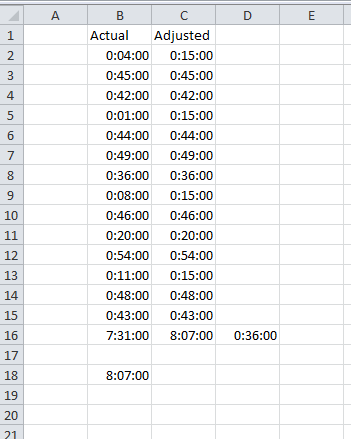
I have a list of times. Some of those times are less than 15 minutes and some are more. My billing floor is 15 minutes. That means that if a task takes me 4 minutes, I still bill 15.
In column C, I have this simple formula:
=MAX(TIME(0,15,0),B2)
That gives me the amount to bill; either 15 minutes or the actual time, whichever is greater. When I sum up that helper column, I get a total that’s 36 minutes more than the actual time. The challenge is to get rid of the helper column. And here’s the answer:
=SUM(B2:B15)+SUMPRODUCT((TIME(0,15,0)-B2:B15>0)*(TIME(0,15,0)-B2:B15))
The SUM simply sums the times and returns 7:31. The SUMPRODUCT section adds up the difference between 15 minutes and the actual time for all those times that are less than 15 minutes. If I use the Ctrl+= to calculate part of the formula, I get
=SUM(B2:B15)+SUMPRODUCT(({TRUE;FALSE;FALSE;TRUE;FALSE;FALSE;FALSE;TRUE;FALSE;FALSE;FALSE;TRUE;FALSE;FALSE})*({0.00763888888888889;-0.0208333333333333;-0.01875;0.00972222222222222;-0.0201388888888889;-0.0236111111111111;-0.0145833333333333;0.00486111111111111;-0.0215277777777778;-0.00347222222222222;-0.0270833333333333;0.00277777777777778;-0.0229166666666667;-0.0194444444444444}))
Yikes, that’s a long one. The first array is a TRUE if the value is less than 15 minutes and a FALSE if not. The second array is the actual difference between the time and 15 minutes. Recall that when TRUE and FALSE are forced to be a number (in this case, we force them to be a number by multiplying them), TRUE becomes 1 and FALSE becomes 0. When the two arrays are multiplied together
=SUM(B2:B15)+SUMPRODUCT({0.00763888888888889;0;0;0.00972222222222222;0;0;0;0.00486111111111111;0;0;0;0.00277777777777778;0;0})
Every value that was greater than zero gets multiplied by a 1, thereby returning itself. Every value that was less than zero gets multiplied by a 0, thereby returning zero. When you sum them all up, you get
=SUM(B2:B15)+0.025
And of course everyone knows that 2.5% of a day is the same as 36 minutes right? One of the bad things about using dates and times in the formula bar is that it converts them all to decimals. But .025 x 24 hours in a day x 60 minutes in an hour does equal 36 minutes. That gets added to the SUM of the actuals and Bob’s your uncle.
If billing per quarter of an hour is usual (as is in our country) you could use the arrayformula:
=SUM(ROUNDUP(96*B2:B15;0))/96
Or exactly like you did it:
{=SUM(IF(ROUNDUP(96*B2:B15;0)=1;1;96*B2:B15))/96}
Why get rid of the helper column if it makes the calculation much clearer and by extension the spreadsheet easier to maintain and support?
We could debate the usefulness of helper columns all day. But for this application, the helper column was hidden for presentation purposes. I’d rather have a slightly more complicated formula than a hidden column.
For this sort of thing (replacing MAX in SUMPRODUCT) I just do it the straightforward way:
{=SUMPRODUCT(IF(TIME(0,15,0) > B2:B15, TIME(0,15,0), B2:B15))}
My last suggestion can be reduced to
{=SUM(IF(ROUNDUP(96*B2:B15;0)=1;1/96;B2:B15))}
The SUMPRODUCT adds no value in {=SUMPRODUCT(IF(TIME(0,15,0) > B2:B15, TIME(0,15,0), B2:B15))}, you might as well just use {=SUM(IF(TIME(0,15,0) > B2:B15, TIME(0,15,0), B2:B15))}
True; I just use SUMPRODUCT instead of SUM by default because it doesn’t cost anything either.