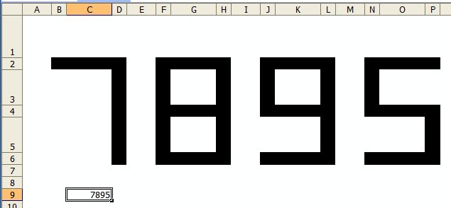
I was reading about seven segment displays over at Sparkfun and thought it would be a fun exercise in Excel. I’m sure it’s been done a million times, but not by me. The first one was VBA based. Type a number into a cell and this code fills cells to display the number as a seven segment display.
|
1 2 3 4 5 6 7 8 9 10 11 12 13 14 15 16 17 18 19 20 21 22 23 24 25 26 27 28 29 30 31 32 33 34 35 36 37 38 39 40 41 42 43 44 45 46 47 48 49 50 51 52 53 54 55 56 57 58 59 60 61 62 63 64 65 66 67 68 69 70 71 72 73 74 75 76 77 78 |
Public Sub ShowSevenSegment(ByVal lInput As Long) Dim sValue As String Dim i As Long, j As Long Dim aDigits(0 To 9) As Variant Dim aRange() As String Dim aRow(0 To 6) As Long, aCol(0 To 6) As Long Dim rSeg As Range Const lDISPCNT As Long = 4 Const lON As Long = vbBlack Const lOFF As Long = vbWhite 'Hold the top left cell for each display ReDim aRange(1 To lDISPCNT) 'Set the on/off for each digit. The order is top, left top, 'right top, middle, left bottom, right bottom, bottom aDigits(0) = Array(lON, lON, lON, lOFF, lON, lON, lON) aDigits(1) = Array(lOFF, lOFF, lON, lOFF, lOFF, lON, lOFF) aDigits(2) = Array(lON, lOFF, lON, lON, lON, lOFF, lON) aDigits(3) = Array(lON, lOFF, lON, lON, lOFF, lON, lON) aDigits(4) = Array(lOFF, lON, lON, lON, lOFF, lON, lOFF) aDigits(5) = Array(lON, lON, lOFF, lON, lOFF, lON, lON) aDigits(6) = Array(lON, lON, lOFF, lON, lON, lON, lON) aDigits(7) = Array(lON, lOFF, lON, lOFF, lOFF, lON, lOFF) aDigits(8) = Array(lON, lON, lON, lON, lON, lON, lON) aDigits(9) = Array(lON, lON, lON, lON, lOFF, lON, lON) 'Set the offset from the top left cell for each of the 'seven segments aRow(0) = 0: aCol(0) = 1 aRow(1) = 1: aCol(1) = 0 aRow(2) = 1: aCol(2) = 2 aRow(3) = 2: aCol(3) = 1 aRow(4) = 3: aCol(4) = 0 aRow(5) = 3: aCol(5) = 2 aRow(6) = 4: aCol(6) = 1 'Set the top left cell for each display For i = 1 To lDISPCNT aRange(i) = Sheet1.Range("B2").Offset(0, (i - 1) * 4).Address Next i 'Truncate and pad the value as necessary If lInput > (10 ^ lDISPCNT) - 1 Then sValue = Left$(lInput, lDISPCNT) Else sValue = Format(lInput, String(lDISPCNT, "0")) End If 'Clear everything Sheet1.Range(aRange(1)).Resize(5, 15).Interior.Color = lOFF 'Loop though the digits For i = 1 To Len(sValue) 'Loop through the on/offs for that digit For j = LBound(aDigits(CLng(Mid$(sValue, i, 1)))) To UBound(aDigits(CLng(Mid$(sValue, i, 1)))) 'get the segment range and set the color Set rSeg = Sheet1.Range(aRange(i)).Offset(aRow(j), aCol(j)) rSeg.Interior.Color = aDigits(CLng(Mid$(sValue, i, 1)))(j) 'color the corners If aDigits(CLng(Mid$(sValue, i, 1)))(j) = lON Then 'for horizontal segments, fill left and right If rSeg.Width > rSeg.Height Then rSeg.Offset(0, -1).Interior.Color = lON rSeg.Offset(0, 1).Interior.Color = lON Else 'for vertical segments, fill up and down rSeg.Offset(-1, 0).Interior.Color = lON rSeg.Offset(1, 0).Interior.Color = lON End If End If Next j Next i End Sub |
OK, it’s really a 13 segment display – the seven segments and six connecting cells. Next, I did the same thing with conditional formatting. I tried to make the conditional formatting formula consistent across the cells, but I just couldn’t. The TRUEs and FALSEs change for each cell depending on if that cell is lit for that number.
Here’s the CF formula for cell H3.
=CHOOSE(MID(TEXT($C$9,"0000"),(COLUMN()+MOD(MOD(MOD(16-COLUMN(),12),8),4))/4,1)+1,TRUE,TRUE,TRUE,TRUE,TRUE,FALSE,FALSE,TRUE,TRUE,TRUE)
H3 is lit for every number except 5 and 6. There’s data validation on the input cell to keep it under five digits. The CF formula is a CHOOSE function with nine TRUEs/FALSEs. To determine which character to represent, I use a MID function after padding the text to four digits. The starting position (second argument of MID) is determine by this:
(COLUMN()+MOD(MOD(MOD(16-COLUMN(),12),8),4))/4,1)
| Column | 16-Column | Mod 12 | Mod 8 | Mod 4 | Column+ | /4 |
|---|---|---|---|---|---|---|
| 2 | 14 | 2 | 2 | 2 | 4 | 1 |
| 3 | 13 | 1 | 1 | 1 | 4 | 1 |
| 4 | 12 | 0 | 0 | 0 | 4 | 1 |
| 6 | 10 | 10 | 2 | 2 | 8 | 2 |
| 7 | 9 | 9 | 1 | 1 | 8 | 2 |
| 8 | 8 | 8 | 0 | 0 | 8 | 2 |
| 10 | 6 | 6 | 6 | 2 | 12 | 3 |
| 11 | 5 | 5 | 5 | 1 | 12 | 3 |
| 12 | 4 | 4 | 4 | 0 | 12 | 3 |
| 14 | 2 | 2 | 2 | 2 | 16 | 4 |
| 15 | 1 | 1 | 1 | 1 | 16 | 4 |
| 16 | 0 | 0 | 0 | 0 | 16 | 4 |
![]() You can download SevenSegment.zip
You can download SevenSegment.zip
This is a great exercise! I appreciate that you showed multiple approaches as it is always good to see things from multiple angles. I decided to take up your exercise and try my hand at it.
I setup a truth table for the numbers, so I could separate that out from the conditional formatting formulas, and looked up the appropriate 1/0 for each number character from the table. Now all I need is one CF formula of Cell Value = 1 to handle all of the cells formulas.
No matter whether the complexity is in the CF formula or on the sheet, it seems that we can’t avoid all of it. It would be interesting to see if any simpler solutions arise from this.
The following single Change event procedure (no other code nor any conditional formatting required) will produce the same results as your posted setup (I have assume the column and row width have been set to their desired widths and heighths)…
Private Sub Worksheet_Change(ByVal Target As Range)Dim X As Long, CellVal As Variant, Digit As Range
If Target.Address = Me.Range("C9").Address Then
CellVal = Target.Value
If CellVal Like "*[!0-9]*" Then
MsgBox "The value you entered is not valid!", vbCritical
Application.EnableEvents = False
Application.Undo
Application.EnableEvents = True
Else
CellVal = Format(CellVal + 0, "0000")
Application.ScreenUpdating = False
For X = 0 To 3
With Range("B2").Offset(, 4 * X)
.Resize(5, 3).Interior.ColorIndex = 1
Select Case Mid(CellVal, 1 + X, 1)
Case 0: .Offset(1, 1).Resize(3, 1).Interior.ColorIndex = 0
Case 1: .Resize(5, 2).Interior.ColorIndex = 0
Case 2: .Offset(1, 0).Resize(1, 2).Interior.ColorIndex = 0
.Offset(3, 1).Resize(1, 2).Interior.ColorIndex = 0
Case 3: .Offset(1, 0).Resize(1, 2).Interior.ColorIndex = 0
.Offset(3, 0).Resize(1, 2).Interior.ColorIndex = 0
Case 4: .Offset(0, 1).Resize(2, 1).Interior.ColorIndex = 0
.Offset(3, 0).Resize(2, 2).Interior.ColorIndex = 0
Case 5: .Offset(1, 1).Resize(1, 2).Interior.ColorIndex = 0
.Offset(3, 0).Resize(1, 2).Interior.ColorIndex = 0
Case 6: .Offset(1, 1).Resize(1, 2).Interior.ColorIndex = 0
.Offset(3, 1).Resize(1, 1).Interior.ColorIndex = 0
Case 7: .Offset(1, 0).Resize(4, 2).Interior.ColorIndex = 0
Case 8: .Offset(1, 1).Resize(1, 1).Interior.ColorIndex = 0
.Offset(3, 1).Resize(1, 1).Interior.ColorIndex = 0
Case 9: .Offset(1, 1).Resize(1, 1).Interior.ColorIndex = 0
.Offset(3, 0).Resize(1, 2).Interior.ColorIndex = 0
End Select
End With
Next
Application.ScreenUpdating = True
End If
End If
End Sub
That’s a lot of code to accomplish a simple task.
A oneliner will do.
With conditional formatting in the range A1:O5 the result will be shown as in Dick’s example.
Formatting conditions:
– when a cell is not empty than black for the seven elements (A2,A4,B1,B3,B5,C2,C4);
– if the adjacent cells are not empty then black for the corner cells between the seven elements (A1,A3,A5,C1,C3,C5). This formatting extended to the Range A1:O5.
In the code I use an asterisk for illustration purposes; I’d prefer to use a space instead.
The number to be shown is in cell A30 (at least in the code below).
Sub M_snb()

     If Len(Format(Val(Cells(30, 1)))) <> 4 Then Exit Sub

    [A1:O5] = [if(iserror(find(address(row(A1:O5),mod(column(A1:O5)-1,4)+1,4),choose(mid(A30,int(column(A1:O5)/4)+1,1)+1,"A2A4B1B5C2C4","C2C4","B1C2B3A4B5","B1C2B3C4B5","A2B3C2C4","A2B1B3C4B5","A2A4B3C4B5","B1C2C4","A2A4B1B3B5C2C4","A2B1B3C2C4"))),"","*")]

End Sub
Nice (although I wouldn’t want to maintain it). Next iteration. Put this formula in A1, then fill right and down to 05.
Then put CF on A1:05 like this
I moved in the input cell to column B because it was wider. The download file will be updated to include @snb’s VBA solution and this one.