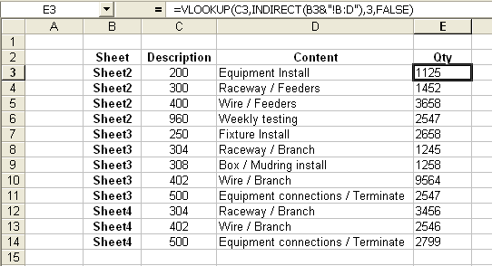
The INDIRECT function can be used to return a range to the VLOOKUP formula. Andy provides this example where the sheet is different for every row, but he doesn’t want to change the formula manually.

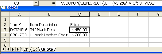
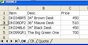
I could see this being useful when the lookup value determines which page the data is on. For example, if you had your inventory on several sheets in a workbook and the inventory item number told you which page it was on. A furniture manufacturer has two classes of inventory, desks and chairs. All the desks start with ‘DK’ and the chairs start with ‘CR’. He could still keep his inventory on two pages and use INDIRECT to point his VLOOKUP to the right list.


With only two inventory classes, there may be a simpler way to do this, but if there were a dozen, this would be a nice shortcut.
Kind of OT:
I always wanted to know which is more efficient approach : a VLOOKUP or Index(Match)
I got used to using Index(Match) and think it as more efficient way because you need to reference 2 Ranges rather than an entire table as with VLOOKUP
Using CHOOSE instead of INDIRECT is much more efficient because CHOOSE is not volatile.
But you are right, CHOOSE gets a bit clumsy with large numbers of choices and there are also the limits of 30 arguments and formula length to consider.
I like this type of use for looking up values from different tables.
However, I have an aversion to large scale use of the volatile function INDIRECT.
I would therefore have table names (dynamic and created with INDEX rather than OFFSET) of DK, CR etc. for as many different categories as required e.g.
=INDEX(DK!$A:$C,1,1):INDEX(DK!$A:$C,COUNTA(DK!$A:$A),3)
I would then insert a defined name USETABLE
=INDIRECT(LEFT(Quote!$A3,2))
Then my lookup formula in Quote B3 would be
=VLOOKUP($B3,usetable,COLUMN(B:B),0)
which I could then drag to C3 and then drag B3 and C3 down the columns.
I may have a totally misconceived idea, but I believe that this would not make as many calls on the INDIRECT function, and therefore give less degradattion in performance when used on fairly large sheets.
I like to use INDIRECT in concert with a data validation dropdown list holding a list of named ranges, then reference that validated cell from the lower cells with INDIRECT then reference those individual cells with VLOOKUP
A B C D
1 LandScape Adjustment SubjectValues AdjustedValue
2 NONE -10000
3 AVG 10000
4 GOOD 15000
5 EXC 20000
Where A1 is the lookup of category lists and A2 et seq contain INDIRECT($A$1) and B2 et seq contain
VLOOKUP(A2,AdjustmentArray,FactorColumn,FALSE)
This is an oversimplification of a pretty powerfull tool for property sales analysis, but maybe you get the idea…
doco
Well that didn’t work worth a @#$#@$@!
A B C D
1 LandScape Adjustment SubjectValue AdjustedValue
2 NONE -10000
3 AVG 10000
4 GOOD 15000
5 EXC 20000
Try this
Hmmmmmmm…
See brief demo HERE
One can avoid the indirect function by using intermediate formulas:
=”=vlookup(a:a,'”&LEFT(A3,2)&”‘!a:c,3,0)”
To evaluate paste values then choose Data|Text to Columns with Delimited and click Finish.
This is recordable and also works when the lookup tables are in closed workbooks.
If current sheet names were in B3:B14, the formulas could be generated in a 3-step process. First create text-valued formulas like this one in E3.
=”=VLOOKUP(C3,'”&B3&”‘!B:D,3,FALSE)”
which would evaluate to
“=VLOOKUP(C3,’Sheet2′!B:D,3,FALSE)”
Copy and paste special as values, then Edit > Replace = with = to ocnvert the text into formulas. This would be better when the worksheets in B3:B14 change infrequently, and it’d pick up changes in worksheet names automatically which the INDIRECT formulas wouldn’t if the B3:B14 entries were constants.
As for Charles Williams points, defined names referring to formulas would be an alternative. They have much more stringent length restrictions than formula cells, but they could be nested.
DefNm0: =CHOOSE(1+INT((X-1)/6),DefNm1,DefNm2,DefNm3,DefNm4)
DefNm1: =CHOOSE(1+MOD(X-1,6),A!$B:$D,B!$B:$D,’C’!$B:$D,D!$B:$D,E!$B:$D,F!$B:$D)
DefNm2: =CHOOSE(1+MOD(X-1,6),G!$B:$D,H!$B:$D,I!$B:$D,J!$B:$D,K!$B:$D,L!$B:$D)
DefNm3: =CHOOSE(1+MOD(X-1,6),M!$B:$D,N!$B:$D,O!$B:$D,P!$B:$D,Q!$B:$D,’R’!$B:$D)
DefNm4: =CHOOSE(1+MOD(X-1,6),S!$B:$D,T!$B:$D,U!$B:$D,V!$B:$D,W!$B:$D,X!$B:$D)
With cell E3 selected, define X as =ThisWorksheetName!$B3. Then with B3:B14 containing worksheet indices rather than names the E3 formula could be replaced by
=VLOOKUP(C3,DefNm0,3,FALSE)
and it should be nonvolatile.
My solution would be to use this lookup formula:
=OFFSET(
INDIRECT(LEFT($A2,2)),
MATCH($A2,OFFSET(INDIRECT(LEFT($A2,2)),0,0,100, 1),0)-1,
MATCH(B$1,OFFSET(INDIRECT(LEFT($A2,2)),0,0, 1,100),0)-1
)
…where column A contains containts the item number to look up and row 1 contains the column header of what needs to be looked up (i.e. “Desc” or “Price” or whatever). The “100? should obviously be changed if the table size merits. Ideally, it would be dynamic based on the spreadsheet, but I would let that go in this application because of the INDIRECT() complication.
But this would require a named range in each lookup sheet named for the sheet and points at the “Item #” lookup column header. I prefer the single cell named range over the entire table because there are fewer complications for row/column insertion deletions. So, long story short, named ranges:
CR = CR!A1
DK = DK!A1
…and so forth.
PS: One pet peeve I have is VLOOKUP() functions that have the third parameter hard-coded (e.g. “3?). It should be something like “COLUMNS(A:C)” — just in case a column gets inserted or moved later on. I don’t know how many times I’ve had to correct a worksheet because someone mangled the table (each person liked “certain” columns together and would rearrange the table, especially when editing was being done).
It’s good to know about and share one’s knowledge about the power of Excel. Yes, with its formulas one can do quite a lot. But, as with so many “solutions” devised with Office products, it seems that the solution tends to define the problem.
In their respective enthusiasm to share how one can “solve” the problem, people seem to have overlooked the obvious. Why does the problem exist in the first place? After all, creating different tables based on what should be nothing more than a value of a key column is a basic no-no in database design!
Together with other common information, the pricing information about chairs and desks (and pens and pencils and…) should be in a single table and not scattered across a myraid of worksheets.
[blockquote]
…basic no-no in database design!
…should be in a single table…
[/blockquote]
You mean a flat file? In the world of handtools this is called a mill bastard – appropriate I think in either case.
While much of what I do with a spreadsheet may be put in one sheet, I have found breaking the larger task into smaller ones is more demonstrable to those I report to as well as make better printouts; which again, satisfies point one. Also, while I have a 24? monitor – and can cover alot of worksheet geography – most can’t; therefore the smaller (non-database) tables accomplish problem solving without creating reports that cannot be read on one screen/printout.
Why go through the excersize if the results cannot be read or understood? The straight line distance between two points being the shortest is oftentimes only true in geometry.
doco
Re The Contrarian’s comments
There’s a fundamental difference between spreadsheets and databases, actually, between relational databases and pretty much all software meant to perform numeric calculations. The data structure described in the original topic is a 3D array. If one doesn’t have relational referencing mechanisms (and Excel lacks them), one needs to use what seems to work best. There are good arguments for using 3D data structures in other spreadsheets and most programming languages. However, since Excel is crippled by it’s lack of general 3D referencing mechanisms (e.g., no INDEX3D which would take 3D references as first argument and sheet index as fourth argument), 3D data structures make much less sense for Excel.
Even so, it’s possible to hack 3D referencing either using INDIRECT with an array of worksheet names or using CHOOSE to select among corresponding ranges on different worksheets. Creating a huge flat file-like single table is arguably trickier and less efficient since it’d require either using a fifth column (3 original columns plus additional component key column plus composite key column) to store the key value or concatenating the columns of component key values to create a composite key value. Difficult as they may be, 3D data structures would be easier to use and more efficient.
Maybe not for The Contrarian, but for me ease and efficiency beat theoretical orthodoxy every time.
>> Why does the problem exist in the first place? After all, creating different tables based on what should be nothing more than a value of a key column is a basic no-no in database design! Together with other common information, the pricing information about chairs and desks (and pens and pencils and…) should be in a single table and not scattered across a myraid of worksheets.
The appropriate solution depends on the problem at hand. While I agree with Contrairian that you are best to keep all of your data in one basket and then create reporting from that one basket, in the real world often you are handed things that do not fit that convenient structure. If I were designing it from scratch then I would go with Contrarians plan every time. But when I get handed something created by others, necessity is often the mother of invention.
With respect to Indirect and Vlookup, there is a place for it but you need to be careful. Indirect is volatile and vlookup is a resource hog (as has already been mentioned). Using them together can be a serious drain on resource. However if used judisciously they are a powerful tool to solve what can be a very tricky problem.
What if the sheet is in another Excel file? I just can’t make a link to “C:somewhere[file]Sheet” and use it.
i have to make one sheet with kind of formul when i change in this sheet all data goes to other sheet automatically
for example
in my general sheet i enter following data
name qty amount
rajan 20 2000
alltech 30 20000
so it automatically goes to sheet 1 (rajan ), and sheet 2(alltech) respectively
Hi
I’ve been searching for the right code all over the web,
Got so many answers, all with errors.
Only here I have found the right coding of how to combine the vlookup() and indirect()
Thank you for that post,
You have saved me lot of hours
Cheers,
Amit
I always try to keep things simple and use named ranges. If its any more complex, use vba.
Great tip; thanks a lot! Worked well for me!
This is actually what I am looking for, but as there isn’t a breakdown on what each element IS or DOES into lamens/english terms I find it difficult to understand.
This is actually something that would fit as I have data on multiple worksheets located in the same are of each worksheet. I then have a master sheet that I would like to enter the name of the worksheet which would bring up the different information based on the worksheet selected.
In a nut shell could someone break the formula into parts so that it is easier to understand? For example:
=VLOOKUP(C3,INDIRECT(B3&”!B:D”),3,FALSE)
Sorry for some reason it submitted without me being able to view and there is no edit option so I can continue my message:
=VLOOKUP(C3,INDIRECT(B3&”!B:D”),3,FALSE)
=VLOOKUP is reference to the VLOOKUP function which searches vertically through a selection
to find information.
C3 is ?
INDIRECT is a reference to the INDIRECT function which points to a certain location
etc.
I would appreciate it if someone could do this for me.
Thank you in advance.
VLOOKUP:
C3 is the first argument – it’s the value you’re looking up.
INDIRECT(…) is the second argument – it’s the range whose first column you’re looking through to find C3
3 is the third column – when C3 is found in the first column, this says to return the 3rd column
FALSE is the fourth argument – it says to only return a value if C3 is found in the first column exactly – close enough isn’t close enough it has to be exact
INDIRECT:
Indirect returns a range based on a string. The string B3&”!B:D” is evaluated to be Sheet2!B:D. Indirect takes that string and turns it into a range reference pointing to the columns B through D on Sheet2.